Machine learning for package users with R (4): Neural Network
These days almost everybody appears to love a variation of Neural Network (NN) -- Deep Learning. I already argued about how Deep Learning works and what kind of parameters characterizes it in the previous post.
A brief trial on a short version of MNIST datasets
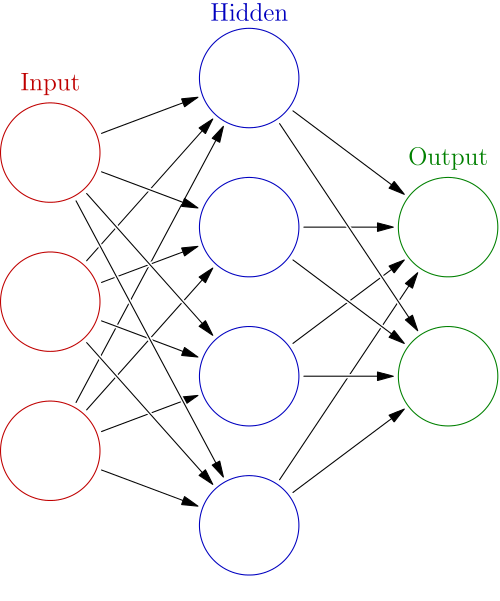
In this post I argue about its origin, usual 3-layers (with only a hidden layer) NN.
> library(nnet)
> train<-read.csv("short_prac_train.csv")
> test<-read.csv("short_prac_test.csv")
> train$label<-as.factor(train$label)
> test$label<-as.factor(test$label)
> train.nnet<-nnet(label~.,train,size=100,decay=0.01,maxit=100,MaxNWts=80000)
# weights:  79510
initial  value 21847.796288
iter  10 value 5304.553496
iter  20 value 3625.223363
iter  30 value 3286.108136
iter  40 value 2882.645985
iter  50 value 2544.534809
iter  60 value 2426.173862
iter  70 value 2300.468337
iter  80 value 2200.327282
iter  90 value 2100.783283
iter 100 value 2042.220475
final  value 2042.220475
stopped after 100 iterations
# took mmmmmmmmmmmmuch long time...

> table(test$label,predict(train.nnet,newdata=test[,-1],type='class'))

     0  1  2  3  4  5  6  7  8  9
  0 93  0  1  0  0  2  2  0  2  0
  1  0 93  1  0  0  2  0  2  2  0
  2  3  3 83  3  1  0  1  2  4  0
  3  2  0  3 79  0  7  1  2  4  2
  4  0  1  1  0 86  2  3  0  1  6
  5  2  0  0  6  2 79  4  1  4  2
  6  2  0  3  0  4  3 87  0  0  1
  7  1  1  1  0  1  0  0 88  2  6
  8  0  0  4  2  1  8  0  2 81  2
  9  0  0  1  2  6  0  0  4  4 83
> sum(diag(table(test$label,predict(train.nnet,newdata=test[,-1],type='class'))))/nrow(test)
[1] 0.852 # OMG, it's low...
Not surprisingly, it's accuracy is low :P) I understand, in principle, NN is hard to be tuned and so that some people call it "a kind of master piece", that means only "masters" can tune it well.
Algorithm summary
As well known, NN is a perceptron with a hidden layer and "back propagation". Very fortunately, the famous textbook ESL clearly explains its algorithm at p.396 as below.
Here is back-propagation in detail for squared error loss. Let
, from (11.5) and let
. Then we have
(11.11)
with derivatives
(11.12)
Given these derivatives, a gradient descent update at the (r + 1)st iteration has the form
(11.13)
where
is the learning rate, discussed below.
Now write (11.12) as
(11.14)
The quantities
and
are "errors" from the current model at the output and hidden layer units, respectively. From their definitions, these errors satisfy
(11.15)
known as the back-propagation equations. Using this, the updates in (11.13) can be implemented with a two-pass algorithm. In the forward pass, the current weights are fixed and the predicted values
are computed from formula (11.5). In the backward pass, the errors
are computed, and then back-propagated via (11.15) to give the errors
. Both sets of errors are then used to compute the gradients for the updates in (11.13), via (11.14).

(wikipedia:en:Artificial_neural_networks)
This algorithm summary says that NN is rather an iterative optimizing procedure than "network". I guess many people regard NN as "network" but from the viewpoint of its algorithm it is merely a two-pass algorithm. This view will be important for understanding how Deep Learning works, as an extension of NN.
How it works on XOR patterns and linearly separable patterns
XOR patterns
OK, let's try it on XOR patterns. I think you already download simple and complex XOR patterns from my GitHub repository. First let's run a parameter tuning routine. Import {nnet} and {caret} packages and run as below.
> library(nnet)
> library(caret)
> xors<-read.table("xor_simple.txt",header=T)
> xors$label<-as.factor(xors$label-1)
> xorc<-read.table("xor_complex.txt",header=T)
> xorc$label<-as.factor(xorc$label-1)

# Tune for simple XOR pattern
> xors.tune<-train(label~.,data=xors,method="nnet",tuneLength=4,maxit=100,trace=F)
Loading required package: class
> print(xors.tune)
Neural Network

100 samples
  2 predictors
  2 classes: '0', '1'

No pre-processing
Resampling: Bootstrapped (25 reps)

Summary of sample sizes: 100, 100, 100, 100, 100, 100, ...

Resampling results across tuning parameters:

  size  decay    Accuracy  Kappa  Accuracy SD  Kappa SD
  1     0        0.659     0.326  0.06         0.099
  1     1e-04    0.65      0.283  0.0466       0.0892
  1     0.00316  0.645     0.284  0.0544       0.0934
  1     0.1      0.643     0.296  0.0611       0.105
  3     0        0.892     0.784  0.0773       0.149
  3     1e-04    0.888     0.772  0.101        0.206
  3     0.00316  0.924     0.846  0.0732       0.146
  3     0.1      0.923     0.845  0.0694       0.139
  5     0        0.913     0.825  0.0512       0.097
  5     1e-04    0.933     0.865  0.0403       0.0802
  5     0.00316  0.951     0.901  0.0405       0.0803
  5     0.1      0.963     0.925  0.0304       0.0612
  7     0        0.925     0.849  0.0394       0.0782
  7     1e-04    0.951     0.901  0.0433       0.086
  7     0.00316  0.95      0.9    0.0431       0.0846
  7     0.1      0.961     0.921  0.0328       0.0657

Accuracy was used to select the optimal model using  the largest value.
The final values used for the model were size = 5 and decay = 0.1.

# Tune for complex XOR pattern
> xorc.tune<-train(label~.,data=xorc,method="nnet",tuneLength=4,maxit=100,trace=F)
> print(xorc.tune)
Neural Network

100 samples
  2 predictors
  2 classes: '0', '1'

No pre-processing
Resampling: Bootstrapped (25 reps)

Summary of sample sizes: 100, 100, 100, 100, 100, 100, ...

Resampling results across tuning parameters:

  size  decay    Accuracy  Kappa   Accuracy SD  Kappa SD
  1     0        0.521     0.0583  0.0808       0.153
  1     1e-04    0.509     0.0332  0.0822       0.152
  1     0.00316  0.531     0.0876  0.0839       0.158
  1     0.1      0.519     0.0638  0.0879       0.176
  3     0        0.652     0.302   0.0985       0.193
  3     1e-04    0.667     0.333   0.0676       0.133
  3     0.00316  0.678     0.359   0.0808       0.148
  3     0.1      0.698     0.394   0.0609       0.119
  5     0        0.677     0.349   0.08         0.161
  5     1e-04    0.673     0.345   0.0758       0.145
  5     0.00316  0.678     0.355   0.0628       0.126
  5     0.1      0.715     0.43    0.079        0.152
  7     0        0.685     0.371   0.0942       0.184
  7     1e-04    0.68      0.361   0.067        0.135
  7     0.00316  0.681     0.363   0.0672       0.131
  7     0.1      0.715     0.431   0.0745       0.144

Accuracy was used to select the optimal model using  the largest value.
The final values used for the model were size = 7 and decay = 0.1.
Now we have a set of best parameters for both simple and complex XOR patterns.
# Set a grid
> px<-seq(-4,4,0.03)
> py<-seq(-4,4,0.03)
> pgrid<-expand.grid(px,py)
> names(pgrid)<-names(xors)[-3]

# Simple XOR pattern
> plot(c(),type='n',xlim=c(-4,4),ylim=c(-4,4))
> par(new=T)
> rect(0,0,4,4,col='#aaaaff')
> par(new=T)
> rect(-4,0,0,4,col='#ffaaaa')
> par(new=T)
> rect(-4,-4,0,0,col='#aaaaff')
> par(new=T)
> rect(0,-4,4,0,col='#ffaaaa')
> par(new=T)
> plot(xors[,-3],col=c(rep('blue',50),rep('red',50)),xlim=c(-4,4),ylim=c(-4,4),pch=19,cex=2.5)
> par(new=T)
> contour(px,py,array(predict(xors.nnet,newdata=pgrid),dim = c(length(px),length(py))),levels = 0.5,drawlabels = T,col='purple',lwd=5,xlim=c(-4,4),ylim=c(-4,4))

# Complex XOR pattern
> plot(c(),type='n',xlim=c(-4,4),ylim=c(-4,4))
> par(new=T)
> rect(0,0,4,4,col='#aaaaff')
> par(new=T)
> rect(-4,0,0,4,col='#ffaaaa')
> par(new=T)
> rect(-4,-4,0,0,col='#aaaaff')
> par(new=T)
> rect(0,-4,4,0,col='#ffaaaa')
> par(new=T)
> plot(xorc[,-3],col=c(rep('blue',50),rep('red',50)),xlim=c(-4,4),ylim=c(-4,4),pch=19,cex=2.5)
> par(new=T)
> contour(px,py,array(predict(xorc.nnet,newdata=pgrid),dim = c(length(px),length(py))),levels = 0.5,drawlabels = T,col='purple',lwd=5,xlim=c(-4,4),ylim=c(-4,4))


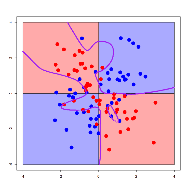
Both look nice. Even in the case of complex XOR pattern, this NN model provides well-smoothed and generalized decision boundaries.
But we can arbitrarily excessively generalize or overfit it to complex XOR pattern with tuning in a bad manner. See below.
# Try to excessively generalize
> xorc.nnet2<-nnet(label~.,xorc,size=2,decay=0.1)
# weights:  9
initial  value 69.974985
iter  10 value 68.637481
iter  20 value 61.866228
iter  30 value 58.071456
final  value 58.067022
converged
> plot(c(),type='n',xlim=c(-4,4),ylim=c(-4,4))
> par(new=T)
> rect(0,0,4,4,col='#aaaaff')
> par(new=T)
> rect(-4,0,0,4,col='#ffaaaa')
> par(new=T)
> rect(-4,-4,0,0,col='#aaaaff')
> par(new=T)
> rect(0,-4,4,0,col='#ffaaaa')
> par(new=T)
> plot(xorc[,-3],col=c(rep('blue',50),rep('red',50)),xlim=c(-4,4),ylim=c(-4,4),pch=19,cex=2.5)
> par(new=T)
> contour(px,py,array(predict(xorc.nnet2,newdata=pgrid),dim = c(length(px),length(py))),levels = 0.5,drawlabels = T,col='purple',lwd=5,xlim=c(-4,4),ylim=c(-4,4))

# Try to overfit
> xorc.nnet3<-nnet(label~.,xorc,size=30,decay=0.01,maxit = 500)
# weights:  121
initial  value 72.772471
iter  10 value 45.654101
iter  20 value 38.793337
iter  30 value 36.433649
iter  40 value 35.542237
iter  50 value 35.151096
iter  60 value 34.962654
iter  70 value 34.787609
iter  80 value 34.711248
iter  90 value 34.677120
iter 100 value 34.647901
iter 110 value 34.627443
iter 120 value 34.617480
iter 130 value 34.611521
iter 140 value 34.607867
iter 150 value 34.605730
iter 160 value 34.604129
iter 170 value 34.602038
iter 180 value 34.600587
iter 190 value 34.599829
iter 200 value 34.599381
iter 210 value 34.599158
iter 220 value 34.599070
iter 230 value 34.598967
iter 240 value 34.598846
iter 250 value 34.598784
iter 260 value 34.598687
iter 270 value 34.598562
iter 280 value 34.598544
final  value 34.598544
converged
> plot(c(),type='n',xlim=c(-4,4),ylim=c(-4,4))
> par(new=T)
> rect(0,0,4,4,col='#aaaaff')
> par(new=T)
> rect(-4,0,0,4,col='#ffaaaa')
> par(new=T)
> rect(-4,-4,0,0,col='#aaaaff')
> par(new=T)
> rect(0,-4,4,0,col='#ffaaaa')
> par(new=T)
> plot(xorc[,-3],col=c(rep('blue',50),rep('red',50)),xlim=c(-4,4),ylim=c(-4,4),pch=19,cex=2.5)
> par(new=T)
> contour(px,py,array(predict(xorc.nnet3,newdata=pgrid),dim = c(length(px),length(py))),levels = 0.5,drawlabels = T,col='purple',lwd=5,xlim=c(-4,4),ylim=c(-4,4))


Hehe, looks crazy! :P) You can well find how NN can be easily tuned worse. So one of my previous colleagues who is an outstanding expert of NN told me "NN is a MASTER PIECE". Yes I agree it.
Linearly separable patterns
> dbi<-read.table("linear_bi.txt",header=T)
> dbi$label<-as.factor(dbi$label)
> summary(dbi)
       x                y         label
 Min.   :0.2112   Min.   :0.177   0:25
 1st Qu.:1.0260   1st Qu.:1.133   1:25
 Median :1.5830   Median :1.616
 Mean   :1.5786   Mean   :1.606
 3rd Qu.:2.0201   3rd Qu.:2.242
 Max.   :3.2749   Max.   :2.994
> dml<-read.table("linear_multi.txt",header=T)
> dml$label<-as.factor(dml$label)
> px2<-seq(-0.5,4.5,0.03)
> py2<-seq(-0.5,4.5,0.03)
> pgrid2<-expand.grid(px2,py2)
> names(pgrid2)<-names(dbi)[-3]
> dbi.tune<-train(label~.,data=dbi,method="nnet",tuneLength=4,maxit=100,trace=F)
> print(dbi.tune)
Neural Network

50 samples
 2 predictors
 2 classes: '0', '1'

No pre-processing
Resampling: Bootstrapped (25 reps)

Summary of sample sizes: 50, 50, 50, 50, 50, 50, ...

Resampling results across tuning parameters:

  size  decay    Accuracy  Kappa  Accuracy SD  Kappa SD
  1     0        0.884     0.763  0.0766       0.165
  1     1e-04    0.878     0.751  0.0798       0.171
  1     0.00316  0.884     0.766  0.0695       0.145
  1     0.1      0.878     0.756  0.0786       0.16
  3     0        0.864     0.724  0.0644       0.129
  3     1e-04    0.874     0.745  0.0722       0.144
  3     0.00316  0.846     0.688  0.0792       0.16
  3     0.1      0.881     0.762  0.0735       0.147
  5     0        0.841     0.676  0.0874       0.179
  5     1e-04    0.834     0.666  0.0984       0.198
  5     0.00316  0.831     0.66   0.0797       0.159
  5     0.1      0.874     0.746  0.0853       0.172
  7     0        0.854     0.705  0.077        0.152
  7     1e-04    0.829     0.653  0.0894       0.18
  7     0.00316  0.818     0.634  0.0904       0.18
  7     0.1      0.874     0.746  0.0853       0.172

Accuracy was used to select the optimal model using  the largest value.
The final values used for the model were size = 1 and decay = 0.00316.
> dml.tune<-train(label~.,data=dml,method="nnet",tuneLength=4,maxit=100,trace=F)
> print(dml.tune)
Neural Network

75 samples
 2 predictors
 3 classes: '0', '1', '2'

No pre-processing
Resampling: Bootstrapped (25 reps)

Summary of sample sizes: 75, 75, 75, 75, 75, 75, ...

Resampling results across tuning parameters:

  size  decay    Accuracy  Kappa  Accuracy SD  Kappa SD
  1     0        0.81      0.711  0.0948       0.145
  1     1e-04    0.828     0.74   0.0582       0.0855
  1     0.00316  0.835     0.75   0.0568       0.0842
  1     0.1      0.784     0.678  0.078        0.108
  3     0        0.823     0.731  0.051        0.0763
  3     1e-04    0.812     0.711  0.0601       0.0978
  3     0.00316  0.82      0.728  0.0728       0.114
  3     0.1      0.835     0.75   0.0544       0.0813
  5     0        0.801     0.701  0.0701       0.103
  5     1e-04    0.81      0.713  0.0601       0.0906
  5     0.00316  0.802     0.7    0.0646       0.102
  5     0.1      0.83      0.743  0.0494       0.0737
  7     0        0.79      0.684  0.0752       0.113
  7     1e-04    0.785     0.676  0.066        0.0974
  7     0.00316  0.804     0.705  0.0629       0.0961
  7     0.1      0.826     0.738  0.0575       0.0841

Accuracy was used to select the optimal model using  the largest value.
The final values used for the model were size = 3 and decay = 0.1.

# Fit NNs
> dbi.nnet<-nnet(label~.,dbi,size=1,decay=dbi.tune$bestTune$decay)
# weights:  5
initial  value 35.776034
iter  10 value 13.686940
iter  20 value 10.696310
iter  30 value 10.639279
iter  40 value 10.636601
final  value 10.636598
converged
> dml.nnet<-nnet(label~.,dml,size=3,decay=dml.tune$bestTune$decay)
# weights:  21
initial  value 96.421336
iter  10 value 47.021366
iter  20 value 38.167857
iter  30 value 37.854914
iter  40 value 37.735454
iter  50 value 37.730520
iter  60 value 37.729962
final  value 37.729953
converged

# 2-classes
> plot(c(),type='n',xlim=c(-0.5,3.5),ylim=c(-0.5,3.5))
> par(new=T)
> polygon(c(-0.5,-0.5,3.5),c(3.5,-0.5,-0.5),col='#aaaaff')
> par(new=T)
> polygon(c(-0.5,3.5,3.5),c(3.5,-0.5,3.5),col='#ffaaaa')
> par(new=T)
> plot(dbi[,-3],pch=19,col=c(rep('blue',25),rep('red',25)),cex=3,xlim=c(-0.5,3.5),ylim=c(-0.5,3.5))
> par(new=T)
> contour(px2,py2,array(predict(dbi.nnet,newdata=pgrid2),dim = c(length(px2),length(py2))),xlim=c(-0.5,3.5),ylim=c(-0.5,3.5),lwd=6,col='purple',levels = 0.5,drawlabels = T)

# 3-classes
> plot(c(),type='n',xlim=c(-0.5,4.5),ylim=c(-0.5,4.5))
> par(new=T)
> polygon(c(-0.5,-0.5,3.5),c(3.5,-0.5,-0.5),col='#aaaaff')
> par(new=T)
> polygon(c(-0.5,3.5,4.5,4.5,1.0,-0.5),c(3.5,-0.5,-0.5,1.0,4.5,4.5),col='#ffaaaa')
> par(new=T)
> polygon(c(1.0,4.5,4.5),c(4.5,1.0,4.5),col='#ccffcc')
> par(new=T)
> plot(dml[,-3],pch=19,col=c(rep('blue',25),rep('red',25),rep('green',25)),cex=3,xlim=c(-0.5,4.5),ylim=c(-0.5,4.5))
> par(new=T)
> contour(px2,py2,array(predict(dml.nnet,newdata=pgrid2,type='class'),dim=c(length(px2),length(py2))),xlim=c(-0.5,4.5),ylim=c(-0.5,4.5),col="purple",lwd=6,drawlabels=T)


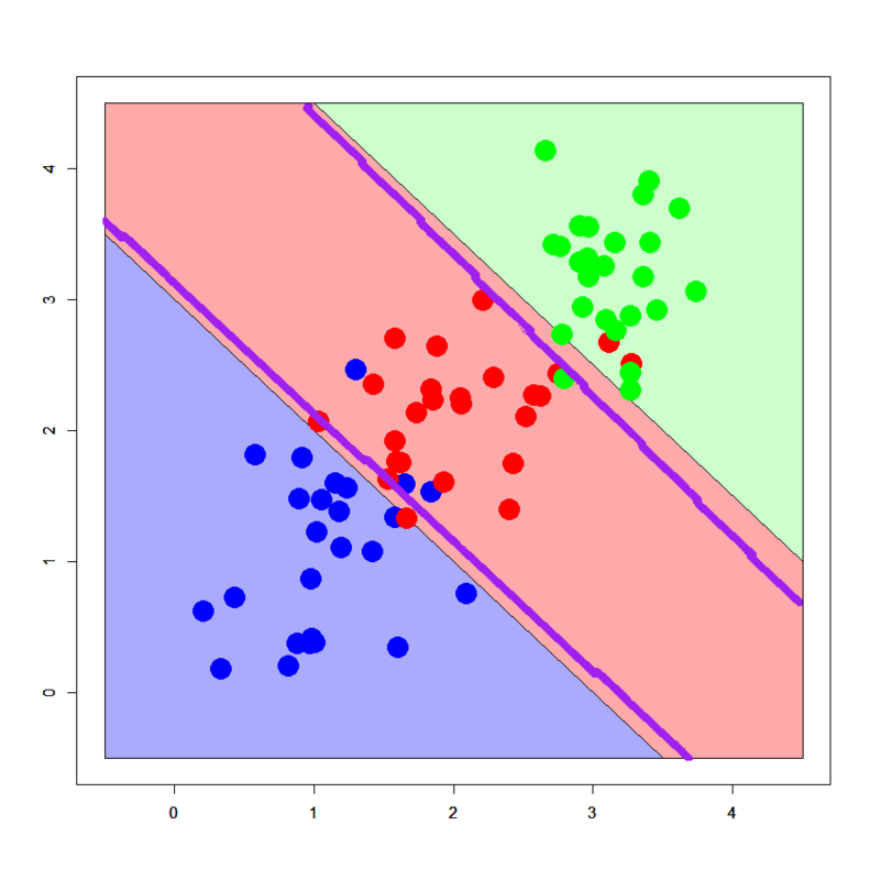
It's confirmed well-tuned NNs successfully draw decision boundaries along the assumed true ones. One of the advantages of NN is, I think, that it's extended from linear perceptron so it can also handle usual linearly separable patterns if correctly tuned.
Conclusions
Lessons we learned here are:
- NN with a single hidden layer is just an iterative optimized learning, rather than "network"
- Performance of NN can be easily affected by parameter tunings
- But NN also work well for both linearly separable and non-separable patterns
I feel these characteristics are taken over by Deep Learning and its family. In that sense, I think we have to seriously review NN with a single hidden layer.
Appendix
h2o.deeplearning() performed as below.
> library(h2o)
> localH2O <- h2o.init(ip = "localhost", port = 54321, startH2O = TRUE, nthreads=7)
> trData<-h2o.importFile(localH2O,path = "short_prac_train.csv")
> tsData<-h2o.importFile(localH2O,path = "short_prac_test.csv")
> res.dl <- h2o.deeplearning(x = 2:785, y = 1, data = trData, activation = "RectifierWithDropout",hidden=c(1024,1024,2048),epochs = 300, adaptive_rate = FALSE, rate=0.01, rate_annealing = 1.0e-6,rate_decay = 1.0, momentum_start = 0.5,momentum_ramp = 5000*18, momentum_stable = 0.99, input_dropout_ratio = 0.2,l1 = 1.0e-5,l2 = 0.0,max_w2 = 15.0, initial_weight_distribution = "Normal",initial_weight_scale = 0.01,nesterov_accelerated_gradient = T, loss = "CrossEntropy", fast_mode = T, diagnostics = T, ignore_const_cols = T,force_load_balance = T)
> pred.dl<-h2o.predict(object=res.dl,newdata=tsData[,-1])
> pred.dl.df<-as.data.frame(pred.dl)
> table(test$label,pred.dl.df[,1])

     0  1  2  3  4  5  6  7  8  9
  0 95  0  1  1  0  0  3  0  0  0
  1  0 99  1  0  0  0  0  0  0  0
  2  0  0 97  0  1  0  0  1  0  1
  3  0  0  1 96  0  2  0  1  0  0
  4  0  1  1  0 96  0  2  0  0  0
  5  0  2  0  3  0 94  1  0  0  0
  6  1  0  0  0  0  1 98  0  0  0
  7  0  0  0  0  3  0  0 97  0  0
  8  0  0  1  3  1  2  0  1 92  0
  9  0  0  0  0  4  0  0  2  0 94
> sum(diag(table(test$label,pred.dl.df[,1])))/nrow(test)
[1] 0.958
Deep Learning worked a little better than random forest, as supposed to be shown in the next post. :D)