Machine learning for package users with R (0): Prologue

Below is the most popular post in this blog that recorded an enormous number of PV and received a lot of comments even here or outside this blog.

In this post, I discussed two aspects of performance of machine learning classifiers: overfitting and generalization. Of course they roughly correspond with bias-variance tradeoff. Low bias models can be easily overfitted and low variance models can be well generalized. In order to describe such a characteristic of each machine learning classifier, I attempted to apply one to a certain fixed dataset; "simple" or "complex" 2D XOR samples.

Indeed I wrote a series of posts running a similar experiment with each classifier, in the Japanese version of my blog. A title of the series can be read "Machine learning for package users with R".

I've heard not a few people request me to translate these posts into English and I agree it would be helpful also for overseas people, so in this series of posts I'll put them into English and discuss some important points for understanding their meaning.

Sample datasets and visualized ones

Prior to the series of experiments, please remember some assumptions; how to tell the classifier is whether "generalized" or "overfitted". In the coming series of posts, I'll use two datasets generated by an R script below.

# Simple XOR pattern
> p11<-cbind(rnorm(n=25,mean=1,sd=0.5),rnorm(n=25,mean=1,sd=0.5))
> p12<-cbind(rnorm(n=25,mean=-1,sd=0.5),rnorm(n=25,mean=1,sd=0.5))
> p13<-cbind(rnorm(n=25,mean=-1,sd=0.5),rnorm(n=25,mean=-1,sd=0.5))
> p14<-cbind(rnorm(n=25,mean=1,sd=0.5),rnorm(n=25,mean=-1,sd=0.5))
> t<-as.factor(c(rep(0,50),rep(1,50)))
> d1<-as.data.frame(cbind(rbind(p11,p13,p12,p14),t))
> names(d1)<-c("x","y","label")

# Complex XOR pattern
> p21<-cbind(rnorm(n=25,mean=1,sd=1),rnorm(n=25,mean=1,sd=1))
> p22<-cbind(rnorm(n=25,mean=-1,sd=1),rnorm(n=25,mean=1,sd=1))
> p23<-cbind(rnorm(n=25,mean=-1,sd=1),rnorm(n=25,mean=-1,sd=1))
> p24<-cbind(rnorm(n=25,mean=1,sd=1),rnorm(n=25,mean=-1,sd=1))
> t<-as.factor(c(rep(0,50),rep(1,50)))
> d2<-as.data.frame(cbind(rbind(p21,p23,p22,p24),t))
> names(d2)<-c("x","y","label")

Obviously, each pattern is a combination of four 2D normal distributions with a fixed standard deviation but placed every quadrant on X-Y plane. "Simple XOR pattern" shows almost no overlap across the distributions but "complex XOR pattern" shows a large amount of overlapping samples. Below are plots of simple and complex XOR patterns with 2 classes, with assumed decision boundaries.

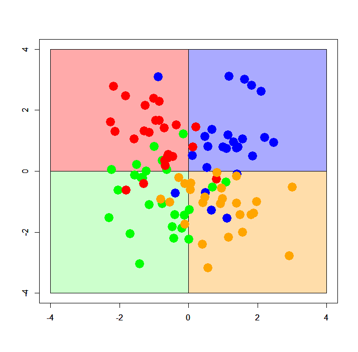
According to the code describing each pattern, we can easily imagine how its assumed decision boundary is; exactly both X and Y axes or straight vertical lines along them. Painted areas show how X-Y plane should be classified by an ideal classifier. If the classifier is well generalized and free from overfitting, its decision boundary must be similar to this painted pattern.

Below are plots of XOR patterns with 4 classes. They also follow the same rule as stated above; but please note that in the case of 4 classes classification its decision boundary can differ from the one with 2 classes. At any rate, in this case the assumed decision boundary is also exactly both X and Y axes or vertical lines along them.

For linear classifiers, I prepare two datasets of linear separable samples with two or three classes. Of course they are to be used for binomial or multinomial logistic regression classifier. Below is an R script generating them.

# Linear separable with 2 classes
> q11<-cbind(rnorm(n=25,mean=1,sd=0.5),rnorm(n=25,mean=1,sd=0.5))
> q12<-cbind(rnorm(n=25,mean=2,sd=0.5),rnorm(n=25,mean=2,sd=0.5))
> t<-as.factor(c(rep(0,25),rep(1,25)))
> dbi<-as.data.frame(cbind(rbind(q11,q12),t))
> names(dbi)<-c("x","y","label")

# Linear separable with 3 classes
> q11<-cbind(rnorm(n=25,mean=1,sd=0.5),rnorm(n=25,mean=1,sd=0.5))
> q12<-cbind(rnorm(n=25,mean=2,sd=0.5),rnorm(n=25,mean=2,sd=0.5))
> q13<-cbind(rnorm(n=25,mean=3,sd=0.5),rnorm(n=25,mean=3,sd=0.5))
> t<-as.factor(c(rep(0,25),rep(1,25),rep(2,25)))
> dmu<-as.data.frame(cbind(rbind(q11,q12,q13),t))
> names(dmu)<-c("x","y","label")

Immediately you'll find that the samples can be easily classified by straight lines; yes, it's why they're called "linearly separable" :) But at the same time we can also test any other kinds of machine learning classifiers in order to check whether they work even for such a linearly separable pattern as well as XOR patterns.

A simple example: Support Vector Machine (SVM) for complex XOR pattern with 4 classes

For example, SVM provides decision boundaries for complex XOR pattern with 4 classes.

As clearly seen, the decision boundaries are approximately parallel to XY axes - in this case I want to call it "well generalized" and "less overfitted", because the decision boundaries don't take in the samples more than needs.

Linear pattern with 3 classes: multinomial logit vs. SVM

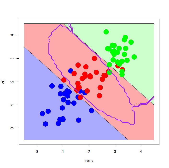
The other interesting example is classification against the linear pattern with 3 classes. For this pattern, not a few classifiers show less generalized and/or much overfitted decision boundaries.

Here we try multinomial logit and SVM.

Left figure is a result of multinomial logit, and right one is that of SVM. It's further interesting - multinomial logit shows well generalized decision boundaries along the assumed boundaries, although SVM shows curious decision boundaries, surrounding #2 class samples circularly.

In future posts

I'll argue about each of popular machine learning classifiers with drawing decision boundaries and comparing them with "assumed boundaries" shown above. I know it'll be interesting. :)

Appendix #1: R scripts drawing plots shown above

# simple XOR with 2 classes
> plot(c(),type='n',xlim=c(-4,4),ylim=c(-4,4))
> par(new=T)
> rect(0,0,4,4,col='#aaaaff')
> par(new=T)
> rect(-4,0,0,4,col='#ffaaaa')
> par(new=T)
> rect(-4,-4,0,0,col='#aaaaff')
> par(new=T)
> rect(0,-4,4,0,col='#ffaaaa')
> par(new=T)
> plot(xors[,-3],col=c(rep('blue',50),rep('red',50)),xlim=c(-4,4),ylim=c(-4,4),pch=19,cex=2.5)

# complex XOR with 2 classes
> plot(c(),type='n',xlim=c(-4,4),ylim=c(-4,4))
> par(new=T)
> rect(0,0,4,4,col='#aaaaff')
> par(new=T)
> rect(-4,0,0,4,col='#ffaaaa')
> par(new=T)
> rect(-4,-4,0,0,col='#aaaaff')
> par(new=T)
> rect(0,-4,4,0,col='#ffaaaa')
> par(new=T)
> plot(xorc[,-3],col=c(rep('blue',50),rep('red',50)),xlim=c(-4,4),ylim=c(-4,4),pch=19,cex=2.5)

# simple XOR with 4 classes
> plot(c(),type='n',xlim=c(-4,4),ylim=c(-4,4))
> par(new=T)
> rect(0,0,4,4,col='#aaaaff')
> par(new=T)
> rect(-4,0,0,4,col='#ffaaaa')
> par(new=T)
> rect(-4,-4,0,0,col='#ccffcc')
> par(new=T)
> rect(0,-4,4,0,col='#ffddaa')
> par(new=T)
> plot(xors[,-3],col=c(rep('blue',25),rep('green',25),rep('red',25),rep('orange',25)),xlim=c(-4,4),ylim=c(-4,4),pch=19,cex=2.5)

# complex XOR with 4 classes
> plot(c(),type='n',xlim=c(-4,4),ylim=c(-4,4))
> par(new=T)
> rect(0,0,4,4,col='#aaaaff')
> par(new=T)
> rect(-4,0,0,4,col='#ffaaaa')
> par(new=T)
> rect(-4,-4,0,0,col='#ccffcc')
> par(new=T)
> rect(0,-4,4,0,col='#ffddaa')
> par(new=T)
> plot(xorc[,-3],col=c(rep('blue',25),rep('green',25),rep('red',25),rep('orange',25)),xlim=c(-4,4),ylim=c(-4,4),pch=19,cex=2.5)

# linearly separable with 2 classes
> plot(c(),type='n',xlim=c(-0.5,3.5),ylim=c(-0.5,3.5))
> par(new=T)
> polygon(c(-0.5,-0.5,3.5),c(3.5,-0.5,-0.5),col='#aaaaff')
> par(new=T)
> polygon(c(-0.5,3.5,3.5),c(3.5,-0.5,3.5),col='#ffaaaa')
> par(new=T)
> plot(dbl[,-3],pch=19,col=c(rep('blue',25),rep('red',25)),cex=3,xlim=c(-0.5,3.5),ylim=c(-0.5,3.5))

# linearly separable with 3 classes
> plot(c(),type='n',xlim=c(-0.5,4.5),ylim=c(-0.5,4.5))
> par(new=T)
> polygon(c(-0.5,-0.5,3.5),c(3.5,-0.5,-0.5),col='#aaaaff')
> par(new=T)
> polygon(c(-0.5,3.5,4.5,4.5,1.0,-0.5),c(3.5,-0.5,-0.5,1.0,4.5,4.5),col='#ffaaaa')
> par(new=T)
> polygon(c(1.0,4.5,4.5),c(4.5,1.0,4.5),col='#ccffcc')
> par(new=T)
> plot(dml[,-3],pch=19,col=c(rep('blue',25),rep('red',25),rep('green',25)),cex=3,xlim=c(-0.5,4.5),ylim=c(-0.5,4.5))

# Prepare a dataset with 4 classes
> xorc$label<-c(rep(0,25),rep(1,25),rep(2,25),rep(3,25))
> xorc$label<-as.factor(xorc$label)

# Tune an SVM model
> xorc.tune<-tune.svm(label~.,data=xorc)
> xorc.tune$best.model

Call:
best.svm(x = label ~ ., data = xorc)


Parameters:
   SVM-Type:  C-classification 
 SVM-Kernel:  radial 
       cost:  1 
      gamma:  0.5 

Number of Support Vectors:  76

# Just fit SVM
> xorc.svm<-svm(label~.,xorc,cost=1,gamma=xorc.tune$best.model$gamma)

# Prepare a grid
> px<-seq(-4,4,0.3)
> py<-seq(-4,4,0.3)
> pgrid<-expand.grid(px,py)
> names(pgrid)<-names(xorc)[1:2]

# Let's plot it
> plot(c(),type='n',xlim=c(-4,4),ylim=c(-4,4))
> par(new=T)
> rect(0,0,4,4,col='#aaaaff')
> par(new=T)
> rect(-4,0,0,4,col='#ffaaaa')
> par(new=T)
> rect(-4,-4,0,0,col='#ccffcc')
> par(new=T)
> rect(0,-4,4,0,col='#ffddaa')
> par(new=T)
> plot(xorc[,-3],col=c(rep('blue',25),rep('green',25),rep('red',25),rep('orange',25)),xlim=c(-4,4),ylim=c(-4,4),pch=19,cex=2.5)
> par(new=T)
> contour(px,py,array(predict(xorc.svm,newdata=pgrid),dim=c(length(px),length(py))),xlim=c(-4,4),ylim=c(-4,4),col="purple",lwd=3,drawlabels=T,levels=c(0.5,1.5,2.5,3.5))

# linearly separable with 3 classes, classified by multinomial logit or SVM
> px2<-seq(-0.5,4.5,0.1)
> py2<-seq(-0.5,4.5,0.1)
> pgrid2<-expand.grid(px2,py2)
> names(pgrid2)<pnames(pgrid)

# Estimate m-logit and SVM
> library(VGAM)
> dml.vglm<-vglm(label~.,dml,family=multinomial)
> out.vglm<-predict(dml.vglm,newdata=pgrid2,type="response")
> out.vglm.class<-matrix(rep(0,dim(out.vglm)[1]),ncol=1)
> for (i in 1:length(out.vglm.class)) {
+      out.vglm.class[i]<-as.numeric(which.max(out.vglm[i,]))-1
+  }

> library(e1071)
> dml.svm<-svm(label~.,dml)

# Let's plot it
> plot(c(),type='n',xlim=c(-0.5,4.5),ylim=c(-0.5,4.5))
> par(new=T)
> polygon(c(-0.5,-0.5,3.5),c(3.5,-0.5,-0.5),col='#aaaaff')
> par(new=T)
> polygon(c(-0.5,3.5,4.5,4.5,1.0,-0.5),c(3.5,-0.5,-0.5,1.0,4.5,4.5),col='#ffaaaa')
> par(new=T)
> polygon(c(1.0,4.5,4.5),c(4.5,1.0,4.5),col='#ccffcc')
> par(new=T)
> plot(dml[,-3],pch=19,col=c(rep('blue',25),rep('red',25),rep('green',25)),cex=3,xlim=c(-0.5,4.5),ylim=c(-0.5,4.5))
> par(new=T)
> contour(px2,py2,array(out.vglm.class,dim=c(length(px2),length(py2))),xlim=c(-0.5,4.5),ylim=c(-0.5,4.5),col="purple",lwd=3,drawlabels=T,levels=c(0.5,1.5))

> plot(c(),type='n',xlim=c(-0.5,4.5),ylim=c(-0.5,4.5))
> par(new=T)
> polygon(c(-0.5,-0.5,3.5),c(3.5,-0.5,-0.5),col='#aaaaff')
> par(new=T)
> polygon(c(-0.5,3.5,4.5,4.5,1.0,-0.5),c(3.5,-0.5,-0.5,1.0,4.5,4.5),col='#ffaaaa')
> par(new=T)
> polygon(c(1.0,4.5,4.5),c(4.5,1.0,4.5),col='#ccffcc')
> par(new=T)
> plot(dml[,-3],pch=19,col=c(rep('blue',25),rep('red',25),rep('green',25)),cex=3,xlim=c(-0.5,4.5),ylim=c(-0.5,4.5))
> par(new=T)
> contour(px2,py2,array(predict(dml.svm,newdata=pgrid2),dim=c(length(px2),length(py2))),xlim=c(-0.5,4.5),ylim=c(-0.5,4.5),col="purple",lwd=3,drawlabels=T,levels=c(0.5,1.5))

Appendix #2: R script to reproduce a short version of MNIST datasets

> dat<-read.csv("prac_train.csv", header=TRUE)
> labels<-dat[,1]
> train_idx<-c()
> for (i in 1:10) {
+     tmp1<-which(labels==(i-1))
+  	tmp2<-sample(tmp1,500,replace=F)
+  	train_idx<-c(train_idx,tmp2)
+  }
> train<-dat[train_idx,]
> dat<-read.csv("prac_test.csv", header=TRUE)
> labels<-dat[,1]
> test_idx<-c()
> for (i in 1:10) {
+     tmp1<-which(labels==(i-1))
+  	tmp2<-sample(tmp1,100,replace=F)
+  	test_idx<-c(test_idx,tmp2)
+  }
> test<-dat[test_idx,]
> write.table(train,file='short_prac_train.csv',quote=F,col.names=T,row.names=F,sep=',')
> write.table(test,file='short_prac_test.csv',quote=F,col.names=T,row.names=F,sep=',')