Undersampling + bagging = better generalized classification for imbalanced dataset
This post is reproduced from a post of my Japanese blog.
A friend of mine, an academic researcher in machine learning field tweeted as below.
imbalanced data に対する対処を勉強していたのだけど,[Wallace et al. ICDM'11] https://t.co/ltQ942lKPm … で「undersampling + bagging をせよ」という結論が出ていた.
— ™ (@tmaehara) July 29, 2017
I've studied how to handle imbalanced data, but I found Wallace et al. ICDM'11 concluded that you should do "undersampling + bagging".
In the other post of my Japanese blog, I argued about how to handle imbalanced data with "class weight" in which cost of negative samples is reduced by a ratio of negative to positive samples in loss function.
However, I thought "undersampling + bagging" would work better, so I would try it here. Please notice that here I only used randomForest {randomForest} in R for this trial just for simplicity and computational cost. If you're interested in any other classifier including deep NN, please try by yourself :P)
Note
If you use Python, already there is a good package for "undersampling + bagging".
Dataset
I prepared a dataset with 250 positive and 3750 negative samples. Please get it from my GitHub repository below.
First, import it as a data frame "d". In addition, let's create a grid to draw decision boundaries.
> px <- seq(-4,4,0.05)
> py <- seq(-4,4,0.05)
> pgrid <- expand.grid(px, py)
> names(pgrid) <- names(d)[-3]
OK, let's proceed.
Class weight
If you use randomForest, what you have to do is just to give a ratio of positive to negative samples to "classwt" argument.
> d.rf <- randomForest(as.factor(label)~., d, classwt=c(1, 3750/250))
> out.rf <- predict(d.rf, newdata=pgrid)
> plot(d[,-3], col=d[,3]+1, xlim=c(-4,4), ylim=c(-4,4), cex=0.5, pch=19)
> par(new=T)
> contour(px, py, array(out.rf, c(length(px), length(py))), levels=0.5, col='purple', lwd=5, drawlabels=F)
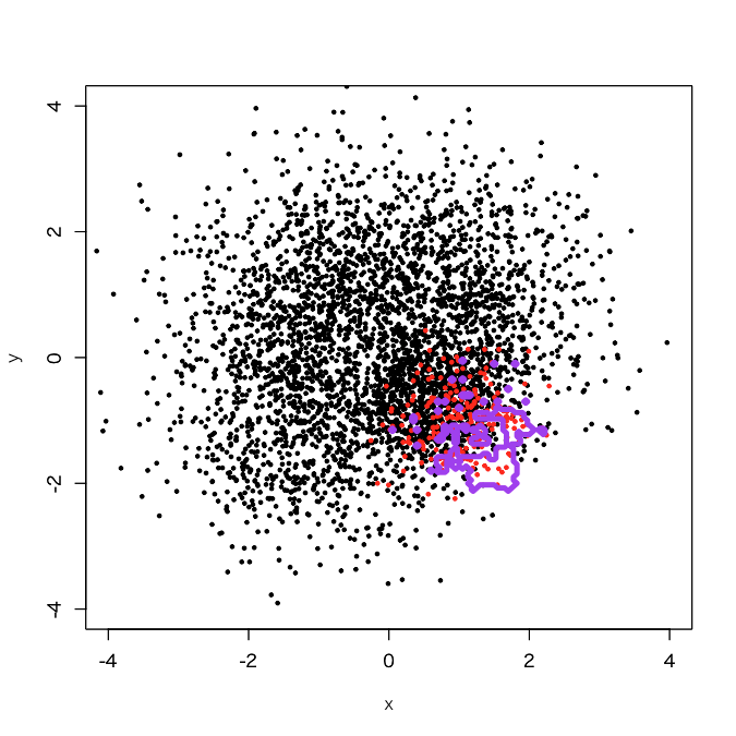
The result was as I expected; a little more expanded decision boundary than its original one.
Undersampling + bagging
First, I tried a bagging with 10 sub-classifiers. Please accept my dirty codes :P)
> outbag.rf <- c()
> for (i in 1:10){
+     set.seed(i)
+     train0 <- d[sample(3750, 250, replace=F),]
+     train1 <- d[3751:4000,]
+     train <- rbind(train0, train1)
+     model <- randomForest(as.factor(label)~., train)
+     tmp <- predict(model, newdata=pgrid)
+     outbag.rf <- cbind(outbag.rf, tmp)
+ }
> outbag.rf.grid <- apply(outbag.rf, 1, mean)-1
> plot(d[,-3], col=d[,3]+1, xlim=c(-4,4), ylim=c(-4,4), cex=0.5, pch=19)
> par(new=T)
> contour(px, py, array(out10.rf.grid, c(length(px), length(py))), levels=0.5, col='purple', lwd=5, drawlabels=F)
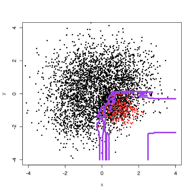
It looks that the classification region of the positive samples got expanded a little bit. How about 50 sub-classifiers?
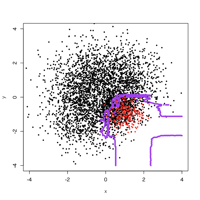
It appears that jaggy parts got reduced. OK, let's try 100 sub-classifiers.
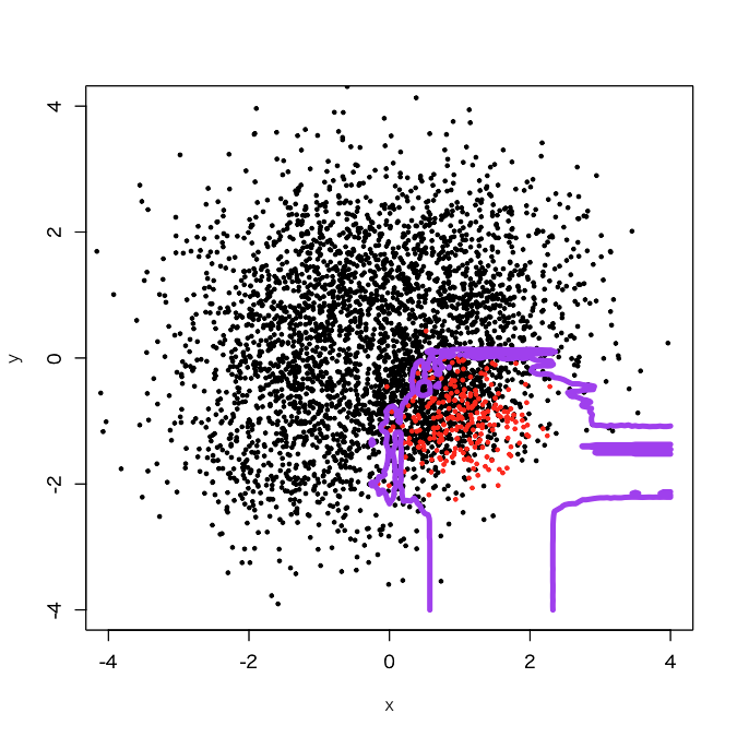
Got it, once it finished.
Advanced: positive samples as embedded into negative samples
The dataset above was generated by a script below.
> set.seed(1001)
> x1 <- cbind(rnorm(1000, 1, 1), rnorm(1000, 1, 1))
> set.seed(1002)
> x2 <- cbind(rnorm(1000, -1, 1), rnorm(1000, 1, 1))
> set.seed(1003)
> x3 <- cbind(rnorm(1000, -1, 1), rnorm(1000, -1, 1))
> set.seed(4001)
> x41 <- cbind(rnorm(250, 0.5, 0.5), rnorm(250, -0.5, 0.5))
> set.seed(4002)
> x42 <- cbind(rnorm(250, 1, 0.5), rnorm(250, -0.5, 0.5))
> set.seed(4003)
> x43 <- cbind(rnorm(250, 0.5, 0.5), rnorm(250, -1, 0.5))
> set.seed(4004)
> x44 <- cbind(rnorm(250, 1, 0.5), rnorm(250, -1, 0.5))
> d <- rbind(x1,x2,x3,x41,x42,x43,x44)
> d <- data.frame(x = d[,1], y = d[,2], label=c(rep(0, 3750), rep(1, 250)))
In short, positive samples in this dataset are concentrated in the lowest and rightmost part of the 4th quadrant, so I think it's natural that we got a result above. Thus, I tried to move the positive samples more inside, as embedded into the negative samples.
> d1 <- d
> d1$label <- c(rep(0,3000), rep(1,250), rep(0,750))
First, let's try "classwt".
> d1.rf <- randomForest(as.factor(label)~., d1, classwt=c(1, 3750/250))
> out.rf <- predict(d1.rf, newdata=pgrid)
> plot(d1[,-3], col=d1[,3]+1, xlim=c(-4,4), ylim=c(-4,4), cex=0.5, pch=19)
> par(new=T)
> contour(px, py, array(out.rf, c(length(px), length(py))), levels=0.5, col='purple', lwd=5, drawlabels=F)
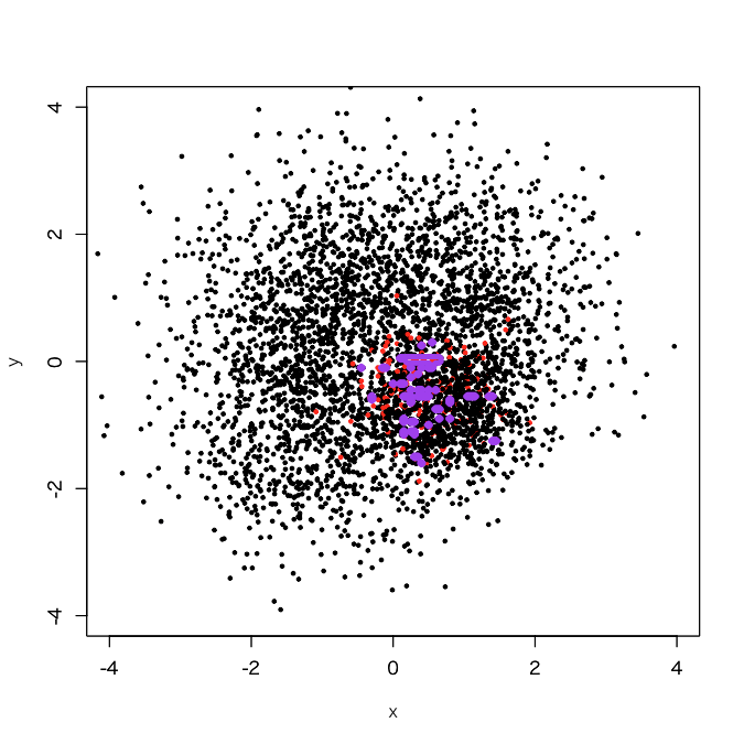
OMG... what a tiny decision boundary, even like overfitting. OK, let's try "undersampling + bagging". For simplicity, I tried 100 sub-classifiers here.
> outbag.rf <- c()
> for (i in 1:100){
+ set.seed(i)
+ train.tmp <- d1[d1$label==0,]
+ train0 <- train.tmp[sample(3750, 250, replace=F),]
+ train1 <- d1[3001:3250,]
+ train <- rbind(train0, train1)
+ model <- randomForest(as.factor(label)~., train)
+ tmp <- predict(model, newdata=pgrid)
+ outbag.rf <- cbind(outbag.rf, tmp)
+ }
> outbag.rf.grid <- apply(outbag.rf, 1, mean)-1
> plot(d1[,-3], col=d1[,3]+1, xlim=c(-4,4), ylim=c(-4,4), cex=0.5, pch=19)
> par(new=T)
> contour(px, py, array(outbag.rf.grid, c(length(px), length(py))), levels=0.5, col='purple', lwd=5, drawlabels=F)
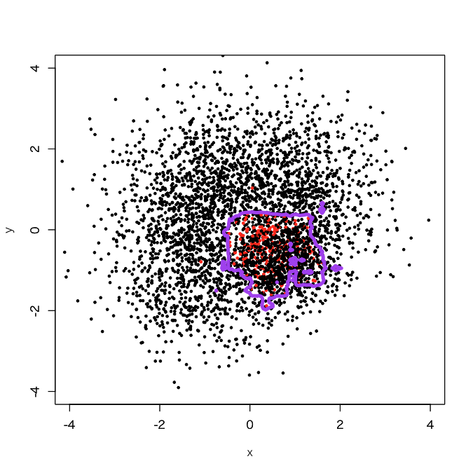
Yes, I didi it. You see a broad decision boundary in the 4th quadrant just near to (0,0), which looks to get a little bit more generalized than usual.
My comment
Two cases clearly showed that "undersampling + bagging" does better than "class weight" in order to get well-generalized decision boundary. To tell the truth, I rather got shocked because "classwt" causes overfitting shown in these two cases...