{mxnet} R package from MXnet, an intuitive Deep Learning framework including CNN & RNN
Actually I've known about MXnet for weeks as one of the most popular library / packages in Kaggler, but just recently I heard bug fix has been almost done and some friends say the latest version looks stable, so at last I installed it.
MXnet is a framework distributed by DMLC, the team also known as a distributor of Xgboost. Now its documentation looks to be completed and even pre-trained models for ImageNet are distributed. I think this should be a good news for R-users loving machine learning... so let's go.
Convolutional Neural Network (CNN)
I believe almost all readers of this blog already know well about Deep Learning and Convolutional Neural Network (CNN)... so here I just show you a brief overview.
CNN is a variant of Deep Learning and it has been well known for its excellent performance of image recognition. In particular, after CNN won ILSVRC 2012, CNN has gotten more and more popular in image recognition. The most recent success of CNN would be AlphaGo, I believe.
Indeed, we already have a lot of implementation of CNN as libraries / packages. For example, a traditional implementation of by Theano requires high skills in coding but it is still popular and widely used. I think PyLearn2 is a little easier but it looks to make many users desperate :P) Torch / Caffe are also great implementation, and Chainer provided some intuitive coding of CNN*1. Finally we see TensorFlow / CNTK, distributed by global IT giants for global standard. Very recently Keras is distributed as a wrapper for both Theano and TensorFlow.
I won't write anything about its theoretical basis and details of the algorithm because I'm never any expert in machine learning nor mathematician :P))) Please search on the web with keywords such as "convolutional neural network" and you'll see too many useful pages, slides or textbooks! At least please make sure about its basic concept, as "input layer --> 'convolution layer x m --> pooling layer' x n --> fully connected layer x p --> output layer", illustrated below.
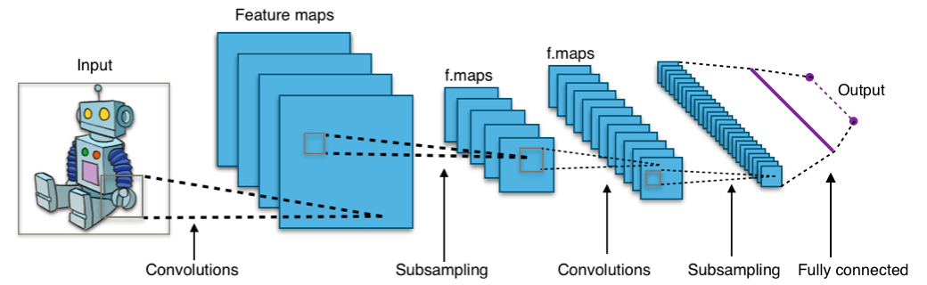
(wikipedia:en:Convolutional_neural_network)
This is very similar to and inspired by visual information processing in the visual cortex of the human brain*2. First input signals are filtered based on orientation selectivity, feature extraction etc.*3, second an invariance of parallel shift is added, finally all processes are integrated.
Classification of the short version of MNIST using R package {mxnet} from MXnet
MXnet is a framework implementing Deep Learning with graph abstraction, very similar to TensorFlow. It's newer than other major libraries / packages of Deep Learning so it has a lot of useful implementation of the pioneers. For example, MXnet can distribute computations, change from CPU to GPU or vice versa easily, provide pre-training models for ImageNet, not only DNN / CNN but also LSTM-RNN, and provide wrappers for Python, R, C++ and Julia which are much popular in data science and/or machine learning community. Even documentation alone looks attractive!
In particular, as far as I've known, there is almost no useful R packages implementing CNN in R, so I think MXnet and its R package {mxnet} would be a great tool for R users. Just personally, Theano requires complicated coding and is a little annoying for me, PyLearn2 is not so easy for me, Caffe / Chainer require GPU instances so I don't like, so I only tried TensorFlow on my own AWS EC2 instance. So MXnet is really great for me because it works on either CPU or GPU, even on local laptops.
OK, let's try the R package {mxnet} in accordance with MXnet's tutorial to see how it works. For your information, my computing environment is as follows:
- Machine: MacBook Pro / OS X El Capitan 10.11.3
- Processors: 3.1 GHz Intel Core i7
- Memory: 16 GB
- R environment: R 3.2.3 / RStudio 0.99.491
From this year I'm a Mac user :P)
Installation
It's very easy, just do as below.
# Installation
> install.packages("drat", repos="https://cran.rstudio.com")
> drat:::addRepo("dmlc")
> install.packages("mxnet")
> library(mxnet)
It's impressive that not devtools but drat is attached. It looks the latest technology in 2016, doesn't it?
Preparing datasets
As raised in the title of this section, let's use the short version of MNIST handwritten digits dataset on my GitHub repository (5,000 rows for training and 1,000 for test). This dataset is not large so I think no classifiers can reach accuracy 0.98. Let's run as below to transform the dataset that can be handle by {mxnet}.
# Data preparation
> train<-read.csv('https://github.com/ozt-ca/tjo.hatenablog.samples/raw/master/r_samples/public_lib/jp/mnist_reproduced/short_prac_train.csv')
> test<-read.csv('https://github.com/ozt-ca/tjo.hatenablog.samples/raw/master/r_samples/public_lib/jp/mnist_reproduced/short_prac_test.csv')
> train<-data.matrix(train)
> test<-data.matrix(test)
> train.x<-train[,-1]
> train.y<-train[,1]
> train.x<-t(train.x/255)
> test_org<-test
> test<-test[,-1]
> test<-t(test/255)
> table(train.y)
train.y
  0   1   2   3   4   5   6   7   8   9
500 500 500 500 500 500 500 500 500 500
Trying Deep Neural Network (DNN)
All right, let's try a classical DNN according to the tutorial. This is merely a multi-layer perceptron with back propagation.
# Deep NN
> data <- mx.symbol.Variable("data")
> fc1 <- mx.symbol.FullyConnected(data, name="fc1", num_hidden=128)
> act1 <- mx.symbol.Activation(fc1, name="relu1", act_type="relu")
> fc2 <- mx.symbol.FullyConnected(act1, name="fc2", num_hidden=64)
> act2 <- mx.symbol.Activation(fc2, name="relu2", act_type="relu")
> fc3 <- mx.symbol.FullyConnected(act2, name="fc3", num_hidden=10)
> softmax <- mx.symbol.SoftmaxOutput(fc3, name="sm")
> devices <- mx.cpu()
> mx.set.seed(0)
> model <- mx.model.FeedForward.create(softmax, X=train.x, y=train.y,
+                                      ctx=devices, num.round=10, array.batch.size=100,
+                                      learning.rate=0.07, momentum=0.9,  eval.metric=mx.metric.accuracy,
+                                      initializer=mx.init.uniform(0.07),
+                                      epoch.end.callback=mx.callback.log.train.metric(100))
Start training with 1 devices
[1] Train-accuracy=0.470204081632653
[2] Train-accuracy=0.8326
[3] Train-accuracy=0.9052
[4] Train-accuracy=0.9278
[5] Train-accuracy=0.9466
[6] Train-accuracy=0.9568
[7] Train-accuracy=0.9646
[8] Train-accuracy=0.9756
[9] Train-accuracy=0.9888
[10] Train-accuracy=0.9926
> preds <- predict(model, test)
> dim(preds)
[1]   10 1000
> pred.label <- max.col(t(preds)) - 1
> table(pred.label)
pred.label
  0   1   2   3   4   5   6   7   8   9
 95 101 101  94 104 104  99 107 102  93
> head(pred.label)
[1] 0 0 0 6 0 0
> table(test_org[,1],pred.label)
   pred.label
      0   1   2   3   4   5   6   7   8   9
  0  94   0   1   0   0   0   3   0   1   1
  1   0 100   0   0   0   0   0   0   0   0
  2   0   0  97   1   1   0   0   1   0   0
  3   0   0   2  91   0   3   0   1   2   1
  4   0   0   0   0  95   0   2   1   0   2
  5   0   1   0   1   0  96   0   0   2   0
  6   1   0   0   0   1   3  94   0   1   0
  7   0   0   0   0   0   0   0 100   0   0
  8   0   0   1   1   1   1   0   0  96   0
  9   0   0   0   0   6   1   0   4   0  89
> sum(diag(table(test_org[,1],pred.label)))/1000
[1] 0.952
Finally we got a result as accuracy 0.952. As mentioned later, this is not good but also not bad.
Trying Convolutional Neural Network (CNN)
OK, now it's time to try CNN, the main dish of this post. According to the code in the tutorial, the CNN should be set as below.

The R script below clearly shows {mxnet} can describe a configuration of convolution, pooling and fully connected layers very intuitively, similarly to Torch or Chainer.
# Convolutional NN
> data <- mx.symbol.Variable('data')
> # first conv
> conv1 <- mx.symbol.Convolution(data=data, kernel=c(5,5), num_filter=20)
> tanh1 <- mx.symbol.Activation(data=conv1, act_type="tanh")
> pool1 <- mx.symbol.Pooling(data=tanh1, pool_type="max",
+                            kernel=c(2,2), stride=c(2,2))
> # second conv
> conv2 <- mx.symbol.Convolution(data=pool1, kernel=c(5,5), num_filter=50)
> tanh2 <- mx.symbol.Activation(data=conv2, act_type="tanh")
> pool2 <- mx.symbol.Pooling(data=tanh2, pool_type="max",
+                            kernel=c(2,2), stride=c(2,2))
> # first fullc
> flatten <- mx.symbol.Flatten(data=pool2)
> fc1 <- mx.symbol.FullyConnected(data=flatten, num_hidden=500)
> tanh3 <- mx.symbol.Activation(data=fc1, act_type="tanh")
> # second fullc
> fc2 <- mx.symbol.FullyConnected(data=tanh3, num_hidden=10)
> # loss
> lenet <- mx.symbol.SoftmaxOutput(data=fc2)
> train.array <- train.x
> dim(train.array) <- c(28, 28, 1, ncol(train.x))
> test.array <- test
> dim(test.array) <- c(28, 28, 1, ncol(test))
> mx.set.seed(0)
> tic <- proc.time()
> model <- mx.model.FeedForward.create(lenet, X=train.array, y=train.y,
+                                      ctx=device.cpu, num.round=20, array.batch.size=100,
+                                      learning.rate=0.05, momentum=0.9, wd=0.00001,
+                                      eval.metric=mx.metric.accuracy,
+                                      epoch.end.callback=mx.callback.log.train.metric(100))
Start training with 1 devices
[1] Train-accuracy=0.0959183673469388
[2] Train-accuracy=0.0902
[3] Train-accuracy=0.0982
[4] Train-accuracy=0.2254
[5] Train-accuracy=0.7958
[6] Train-accuracy=0.9074
[7] Train-accuracy=0.942
[8] Train-accuracy=0.9626
[9] Train-accuracy=0.9762
[10] Train-accuracy=0.9814
[11] Train-accuracy=0.9846
[12] Train-accuracy=0.988
[13] Train-accuracy=0.993
[14] Train-accuracy=0.996
[15] Train-accuracy=0.9988
[16] Train-accuracy=0.9996
[17] Train-accuracy=0.9996
[18] Train-accuracy=1
[19] Train-accuracy=1
[20] Train-accuracy=1
> print(proc.time() - tic)
   ユーザ   システム       経過
   270.122      1.216    234.877
> preds <- predict(model, test.array)
> pred.label <- max.col(t(preds)) - 1
> table(test_org[,1],pred.label)
   pred.label
      0   1   2   3   4   5   6   7   8   9
  0  97   0   0   0   0   0   3   0   0   0
  1   0 100   0   0   0   0   0   0   0   0
  2   0   0  99   0   0   0   0   1   0   0
  3   0   0   1  96   0   0   0   0   2   1
  4   0   0   0   0  97   0   1   1   0   1
  5   0   0   0   0   0  98   1   0   1   0
  6   1   0   0   0   0   1  98   0   0   0
  7   0   1   1   0   1   0   0  96   0   1
  8   0   0   1   0   0   0   0   0  99   0
  9   0   0   0   0   2   1   0   0   1  96
> sum(diag(table(test_org[,1],pred.label)))/1000
[1] 0.976
Accuracy 0.976 was the performance of our simple CNN. In the tutorial, num.round is set to 1 but I changed it to 20*4. Computation time was 270 sec, further shorter than the case with {h2o}. It's great! :O)
As just a trial, 4 samples of '9' digit in the test dataset that were incorrectly predicted as 4, 5 or 8 are visualized below.

Hey, who can identify them :P))) They are too ambiguous to be recognized correctly even by our brief CNN based on the tutorial of {mxnet}. Of course I know it's a fun for Kagglers to recognize such weird digit samples in MNIST.
Comparison to other methods
Accuracy 0.976 on the short version of MNIST means the best benchmark ever in my blog. Let's review other benchmarks given by other classifiers.
Random Forest
> train<-read.csv('https://github.com/ozt-ca/tjo.hatenablog.samples/raw/master/r_samples/public_lib/jp/mnist_reproduced/short_prac_train.csv')
> test<-read.csv('https://github.com/ozt-ca/tjo.hatenablog.samples/raw/master/r_samples/public_lib/jp/mnist_reproduced/short_prac_test.csv')
> train$label<-as.factor(train$label)
> test$label<-as.factor(test$label)

> library(randomForest)
> train.rf<-randomForest(label~.,train)
> table(test$label,predict(train.rf,newdata=test[,-1]))

     0  1  2  3  4  5  6  7  8  9
  0 96  0  0  0  0  0  3  0  1  0
  1  0 99  0  0  0  0  0  0  1  0
  2  0  0 96  1  1  0  1  1  0  0
  3  0  0  2 87  0  4  1  1  3  2
  4  0  0  0  0 96  0  1  0  0  3
  5  1  2  0  1  0 94  2  0  0  0
  6  0  0  1  0  1  2 95  0  1  0
  7  0  2  0  0  1  0  0 93  0  4
  8  0  0  1  0  0  0  0  0 99  0
  9  0  0  0  0  2  1  0  1  0 96
> sum(diag(table(test$label,predict(train.rf,newdata=test[,-1]))))/nrow(test)
[1] 0.951
Accuracy was 0.951, but it's without parameter tuning by tuneRF (omitted for computation resource). It can be improved I think.
Xgboost
> train<-read.csv('https://github.com/ozt-ca/tjo.hatenablog.samples/raw/master/r_samples/public_lib/jp/mnist_reproduced/short_prac_train.csv')
> test<-read.csv('https://github.com/ozt-ca/tjo.hatenablog.samples/raw/master/r_samples/public_lib/jp/mnist_reproduced/short_prac_test.csv')

> library(xgboost)
> library(Matrix)
> train.mx<-sparse.model.matrix(label~., train)
> test.mx<-sparse.model.matrix(label~., test)
> dtrain<-xgb.DMatrix(train.mx, label=train$label)
> dtest<-xgb.DMatrix(test.mx, label=test$label)
> train.gdbt<-xgb.train(params=list(objective="multi:softmax", num_class=10, eval_metric="mlogloss", eta=0.3, max_depth=5, subsample=1, colsample_bytree=0.5), data=dtrain, nrounds=70, watchlist=list(train=dtrain,test=dtest))
[0]	train-mlogloss:1.439942	test-mlogloss:1.488160
[1]	train-mlogloss:1.083675	test-mlogloss:1.177975
[2]	train-mlogloss:0.854107	test-mlogloss:0.977648
# ... omitted ...
[67]	train-mlogloss:0.004172	test-mlogloss:0.176068
[68]	train-mlogloss:0.004088	test-mlogloss:0.176044
[69]	train-mlogloss:0.004010	test-mlogloss:0.176004
> table(test$label,predict(train.gdbt,newdata=dtest))

     0  1  2  3  4  5  6  7  8  9
  0 95  0  0  1  0  0  3  0  1  0
  1  0 99  0  0  0  0  0  1  0  0
  2  0  0 96  2  0  0  1  1  0  0
  3  0  0  1 93  0  0  0  1  2  3
  4  0  0  1  1 95  0  1  0  0  2
  5  0  1  0  1  0 98  0  0  0  0
  6  0  0  1  0  1  2 95  0  1  0
  7  0  0  0  0  1  0  0 96  0  3
  8  0  4  1  0  1  0  0  0 93  1
  9  0  0  0  0  4  1  0  2  0 93
> sum(diag(table(test$label,predict(train.gdbt,newdata=dtest))))/nrow(test)
[1] 0.953
Accuracy was 0.953. This was a result through intensive parameter tuning, so it may be plausible.
DNN by {h2o}
> train<-read.csv('https://github.com/ozt-ca/tjo.hatenablog.samples/raw/master/r_samples/public_lib/jp/mnist_reproduced/short_prac_train.csv')
> test<-read.csv('https://github.com/ozt-ca/tjo.hatenablog.samples/raw/master/r_samples/public_lib/jp/mnist_reproduced/short_prac_test.csv')
> train$label<-as.factor(train$label)
> test$label<-as.factor(test$label)

> library(h2o)
> localH2O <- h2o.init(ip = "localhost", port = 54321, startH2O = TRUE, nthreads=3)
> trData<-as.h2o(train)
> tsData<-as.h2o(test)
> res.dl <- h2o.deeplearning(x = 2:785, y = 1, training_frame = trData, activation = "RectifierWithDropout",hidden=c(1024,1024,2048),epochs = 300, adaptive_rate = FALSE, rate=0.01, rate_annealing = 1.0e-6,rate_decay = 1.0, momentum_start = 0.5,momentum_ramp = 5000*18, momentum_stable = 0.99, input_dropout_ratio = 0.2,l1 = 1.0e-5,l2 = 0.0,max_w2 = 15.0, initial_weight_distribution = "Normal",initial_weight_scale = 0.01,nesterov_accelerated_gradient = T, loss = "CrossEntropy", fast_mode = T, diagnostics = T, ignore_const_cols = T,force_load_balance = T)
> pred<-h2o.predict(res.dl,tsData[,-1])
> pred.df<-as.data.frame(pred)
> table(test$label,pred.df[,1])

      0   1   2   3   4   5   6   7   8   9
  0  96   0   1   0   0   0   2   1   0   0
  1   0 100   0   0   0   0   0   0   0   0
  2   0   0  97   0   2   0   0   1   0   0
  3   0   0   1  93   0   4   0   1   0   1
  4   0   2   1   0  93   0   0   1   1   2
  5   0   0   0   1   0  99   0   0   0   0
  6   1   0   0   0   0   2  97   0   0   0
  7   0   0   0   0   1   0   0  96   0   3
  8   0   0   1   1   1   2   0   0  95   0
  9   0   0   0   0   2   0   0   2   0  96
> sum(diag(table(test$label,pred.df[,1])))/nrow(test)
[1] 0.962
Accuracy was 0.962, through the best parameter tuning shown in a certain slideshare by H2O... our brief CNN by {mxnet} even overtook it. This fact means even a simple CNN is better than the best-tuned DNN. It's plausible these days almost everybody loves to use CNN for image recognition.
My comments
The first point is its usability. Changing CPU to GPU or vice versa is very easy, and its coding is intuitive to compose almost any kind of Deep Net with just specifying parameters. The second point is its speed. {mxnet} is very fast as well as {xgboost} from the same DMLC. It's even further faster than DNN by {h2o}, based Java VMs.
The more important point is that we can run CNN both in R and Python in almost the same manner. This is a huge advantage for R / Python users, in particular people doing ad-hoc analysis; in several business missions, we often have to build a prototype on a local machine like "a Kaggle competition only by me" and if it's successful we would implement it onto products. In such cases, data scientists like me often use R first, and Python second.
In my personal opinion, R is better than Python for building prototypes because manipulating variables is much easier in R than other languages, but R is not good for implementation on products. On the other hand, Python is vice versa... so a lot of data scientists like me love both R and Python. Actually in my previous job, once I built a prototype of a machine learning system in R and then I implemented it in Python for a product with Xgboost. MXnet enables us to run almost the same procedure for CNN. This is very much helpful for all R users, I believe.
Of course some problems still remain; in particular, parameter tuning of CNN is an incredibly annoying job and even an issue in machine learning researches. As far as I've heard, there are some academic studies in which parameters are optimized through Bayesian sampling and/or Monte Carlo search... I can't imagine how long it will take on local machines. Even with MXnet, we have to keep on struggling with such a kind of remaining problems.
At any rate, I think MXnet can be a strong candidate of Deep Learning library that can compete Chainer / TensorFlow. I hope there will be further interesting and useful libraries / packages of Deep Learning in the future.
In a coming post, I'm planning the other framework in MXnet such as LSTM-RNN, but it requires my own further understanding of its theoretical background. I won't tell when the post will be published :P)
Appendix 1
When activation function is replaced with ReLU, its performance got improved.
> data <- mx.symbol.Variable("data")
> devices<-mx.cpu()
> # first conv
> conv1 <- mx.symbol.Convolution(data=data, kernel=c(5,5), num_filter=20)
> tanh1 <- mx.symbol.Activation(data=conv1, act_type="relu")
> pool1 <- mx.symbol.Pooling(data=tanh1, pool_type="max",
+                            kernel=c(2,2), stride=c(2,2))
> drop1 <- mx.symbol.Dropout(data=pool1,p=0.5)
> # second conv
> conv2 <- mx.symbol.Convolution(data=drop1, kernel=c(5,5), num_filter=50)
> tanh2 <- mx.symbol.Activation(data=conv2, act_type="relu")
> pool2 <- mx.symbol.Pooling(data=tanh2, pool_type="max",
+                            kernel=c(2,2), stride=c(2,2))
> drop2 <- mx.symbol.Dropout(data=pool2,p=0.5)
> # first fullc
> flatten <- mx.symbol.Flatten(data=drop2)
> fc1 <- mx.symbol.FullyConnected(data=flatten, num_hidden=500)
> tanh4 <- mx.symbol.Activation(data=fc1, act_type="relu")
> drop4 <- mx.symbol.Dropout(data=tanh4,p=0.5)
> # second fullc
> fc2 <- mx.symbol.FullyConnected(data=drop4, num_hidden=10)
> # loss
> lenet <- mx.symbol.SoftmaxOutput(data=fc2)
> train.array <- train.x
> dim(train.array) <- c(28, 28, 1, ncol(train.x))
> test.array <- test
> dim(test.array) <- c(28, 28, 1, ncol(test))
> mx.set.seed(0)
> tic <- proc.time()
> model <- mx.model.FeedForward.create(lenet, X=train.array, y=train.y,
+                                      ctx=devices, num.round=60, array.batch.size=100,
+                                      learning.rate=0.05, momentum=0.9, wd=0.00001,
+                                      eval.metric=mx.metric.accuracy,
+                                      epoch.end.callback=mx.callback.log.train.metric(100))
Start training with 1 devices
[1] Train-accuracy=0.0975510204081633
[2] Train-accuracy=0.0906
[3] Train-accuracy=0.09
[4] Train-accuracy=0.0952
[5] Train-accuracy=0.1312
[6] Train-accuracy=0.5612
[7] Train-accuracy=0.8384
[8] Train-accuracy=0.8974
[9] Train-accuracy=0.9156
[10] Train-accuracy=0.9296
[11] Train-accuracy=0.9366
[12] Train-accuracy=0.9436
[13] Train-accuracy=0.9452
[14] Train-accuracy=0.943
[15] Train-accuracy=0.9504
[16] Train-accuracy=0.9566
[17] Train-accuracy=0.955
[18] Train-accuracy=0.9634
[19] Train-accuracy=0.9636
[20] Train-accuracy=0.9594
[21] Train-accuracy=0.9624
[22] Train-accuracy=0.9644
[23] Train-accuracy=0.964
[24] Train-accuracy=0.9628
[25] Train-accuracy=0.9658
[26] Train-accuracy=0.9674
[27] Train-accuracy=0.971
[28] Train-accuracy=0.9692
[29] Train-accuracy=0.9716
[30] Train-accuracy=0.9766
[31] Train-accuracy=0.9712
[32] Train-accuracy=0.9758
[33] Train-accuracy=0.9694
[34] Train-accuracy=0.9694
[35] Train-accuracy=0.9688
[36] Train-accuracy=0.9768
[37] Train-accuracy=0.9728
[38] Train-accuracy=0.9744
[39] Train-accuracy=0.971
[40] Train-accuracy=0.9722
[41] Train-accuracy=0.9746
[42] Train-accuracy=0.9758
[43] Train-accuracy=0.9794
[44] Train-accuracy=0.9756
[45] Train-accuracy=0.9746
[46] Train-accuracy=0.9778
[47] Train-accuracy=0.9766
[48] Train-accuracy=0.9768
[49] Train-accuracy=0.976799999999999
[50] Train-accuracy=0.977399999999999
[51] Train-accuracy=0.9786
[52] Train-accuracy=0.978
[53] Train-accuracy=0.9786
[54] Train-accuracy=0.9774
[55] Train-accuracy=0.9808
[56] Train-accuracy=0.976
[57] Train-accuracy=0.9762
[58] Train-accuracy=0.9794
[59] Train-accuracy=0.978
[60] Train-accuracy=0.9822
> print(proc.time() - tic)
   ユーザ   システム       経過
   784.666      3.767    677.921
> preds <- predict(model, test.array)
> pred.label <- max.col(t(preds)) - 1
> table(test_org[,1],pred.label)
   pred.label
      0   1   2   3   4   5   6   7   8   9
  0  99   0   0   0   0   0   1   0   0   0
  1   0  99   0   0   1   0   0   0   0   0
  2   0   0  98   0   0   0   0   1   1   0
  3   0   0   0  98   0   1   0   0   1   0
  4   0   2   0   0  97   0   1   0   0   0
  5   0   0   0   0   0  99   1   0   0   0
  6   0   0   0   0   0   0 100   0   0   0
  7   0   0   0   0   0   0   0  99   1   0
  8   0   0   0   0   0   0   0   0 100   0
  9   0   0   0   0   2   0   0   0   0  98
> sum(diag(table(test_org[,1],pred.label)))/1000
[1] 0.987
Finally we got accuracy 0.987, overtaking our estimated maximum 0.98.
*1:It's very easy because we only have to write parameters of CNN simply
*2:Actually I was a postdoc researcher in visual information processing of the human brain before joining data science field
*3:Similar to information processing at receptive fields
*4:If it remains, all predicted labels will be '5'...