Machine learning for package users with R (2): Logistic Regression

I think a lot of people love logistic regression because it's pretty light and fast. But we know it's just a linear classifying function -- I mean it's only for linearly separable patterns, not linearly non-separable ones.

f:id:TJO:20150402143508p:plain:w350

It's primary idea is simple: fitting binomial dependent variable with logit function. But its advantage is great even though mainly it works only for linearly separable patterns.

A brief trial on a short version of MNIST datasets

First I tried vglm() function of {VGAM} package on short MNIST dataset.

> train<-read.csv("short_prac_train.csv")
> test<-read.csv("short_prac_test.csv")
> train$label<-as.factor(train$label)
> test$label<-as.factor(test$label)
> library(VGAM)
> train.vglm<-vglm(label~.,train,family=multinomial)
Error in if (min(ans) == 0 || max(ans) == 1) warning("fitted probabilities numerically 0 or 1 occurred") : 
  missing value where TRUE/FALSE needed
In addition: Warning messages:
1: In slot(family, "linkinv")(eta, extra) :
  fitted probabilities numerically 0 or 1 occurred
2: In tfun(mu = mu, y = y, w = w, res = FALSE, eta = eta, extra) :
  fitted values close to 0 or 1
3: In slot(family, "linkinv")(eta, extra) :
  there are NAs in eta in slot inverse
4: In slot(family, "linkinv")(eta, extra) :
  there are NAs here in slot linkinv

OMG, it got crashed maybe because of out of memory :( Let's skip this part and see its algorithm.

Algorithm summary

The Elements of Statistical Learning: Data Mining, Inference, and Prediction

I think I should have cite this well-known but amazing textbook, ESL, in the previous post... for understanding an algorithm of logistic regression, just see 4.4.1 section of the textbook.

In short, it's merely a fitting procedure by maximum likelihood with binomial (or multinomial) distribution. If you want to implement from scratch, you have to understand how iteratively reweighted least squares (IRLS) algorithm works.

As a result of some calculation, finally we have two important steps in order to get estimates of parameters $\beta$ .

$\beta^{new} = (\mathbf{X}^T\mathbf{WX})^{-1}\mathbf{X}^T\mathbf{Wz}$

$\mathbf{z} = \mathbf{X}\beta^{old} + \mathbf{W}^{-1} (\mathbf{y} - \mathbf{p})$

Through them, $\mathbf{p}, \mathbf{W}, \mathbf{z}$ change at each iteration. With repeating these steps, we can solve a weighted least mean square problem below.

$\beta^{new} \leftarrow argmin_{\beta} (\mathbf{z} - \mathbf{X}\beta)^T \mathbf{X} (\mathbf{z} - \mathbf{X}\beta)$

This algorithm is not so complicated that everybody can easily implement e.g. in Python, Java or any other language. Even you can implement in R, but I guess it would be heavy :P)

How it works on XOR patterns and linearly separable patterns

XOR patterns

In principle, logistic regression doesn't work for linearly non-separable patterns. Please download "xor_simple.txt", "xor_complex.txt" from my GitHub repository and run on R as below.

<a href="https://github.com/ozt-ca/tjo.hatenablog.samples/tree/master/r_samples/public_lib/jp">ozt-ca/tjo.hatenablog.samples</a>

> xors<-read.table("xor_simple.txt",header=T)
> xorc<-read.table("xor_complex.txt",header=T)
> xors$label<-as.factor(xors$label)
> xorc$label<-as.factor(xorc$label)
> xors.glm1<-glm(label~.,xors,family=binomial) # simple XOR
> xorc.glm1<-glm(label~.,xorc,family=binomial) # complex XOR
# Prepare a grid
> px<-seq(-4,4,0.03)
> py<-seq(-4,4,0.03)
> pgrid<-expand.grid(px,py)
> names(pgrid)<-names(xors)[-3]
# Plot decision boundary for simple XOR pattern
> plot(c(),type='n',xlim=c(-4,4),ylim=c(-4,4))
> par(new=T)
> rect(0,0,4,4,col='#aaaaff')
> par(new=T)
> rect(-4,0,0,4,col='#ffaaaa')
> par(new=T)
> rect(-4,-4,0,0,col='#aaaaff')
> par(new=T)
> rect(0,-4,4,0,col='#ffaaaa')
> par(new=T)
> plot(xors[,-3],col=c(rep('blue',50),rep('red',50)),xlim=c(-4,4),ylim=c(-4,4),pch=19,cex=2.5)
> par(new=T)
> contour(px,py,array(predict(xors.glm1,newdata=pgrid,type='response'),dim = c(length(px),length(py))),levels = 0.5,drawlabels = T,col='purple',lwd=3,xlim=c(-4,4),ylim=c(-4,4))
# Plot decision boundary for complex XOR pattern
> plot(c(),type='n',xlim=c(-4,4),ylim=c(-4,4))
> par(new=T)
> rect(0,0,4,4,col='#aaaaff')
> par(new=T)
> rect(-4,0,0,4,col='#ffaaaa')
> par(new=T)
> rect(-4,-4,0,0,col='#aaaaff')
> par(new=T)
> rect(0,-4,4,0,col='#ffaaaa')
> par(new=T)
> plot(xorc[,-3],col=c(rep('blue',50),rep('red',50)),xlim=c(-4,4),ylim=c(-4,4),pch=19,cex=2.5)
> par(new=T)
> contour(px,py,array(predict(xorc.glm1,newdata=pgrid,type='response'),dim = c(length(px),length(py))),levels = 0.5,drawlabels = T,col='purple',lwd=3,xlim=c(-4,4),ylim=c(-4,4))

f:id:TJO:20150325173314p:plain

f:id:TJO:20150325173913p:plain

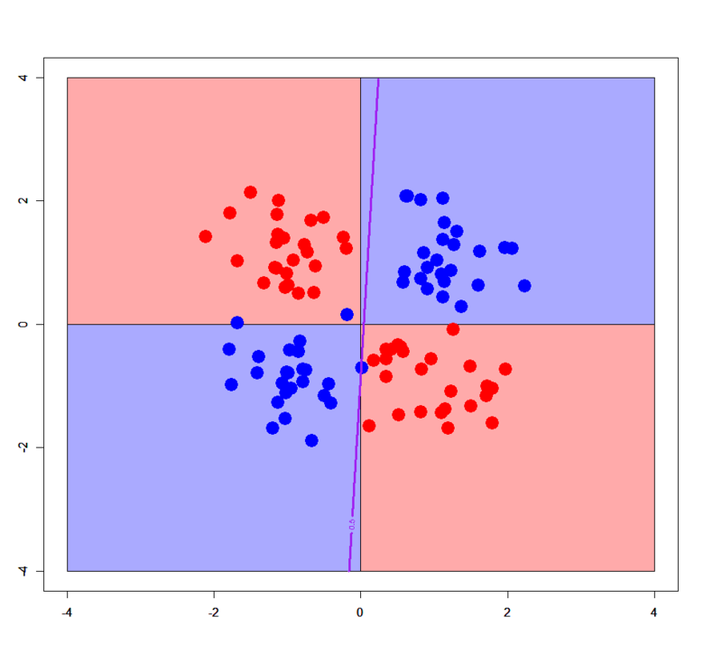
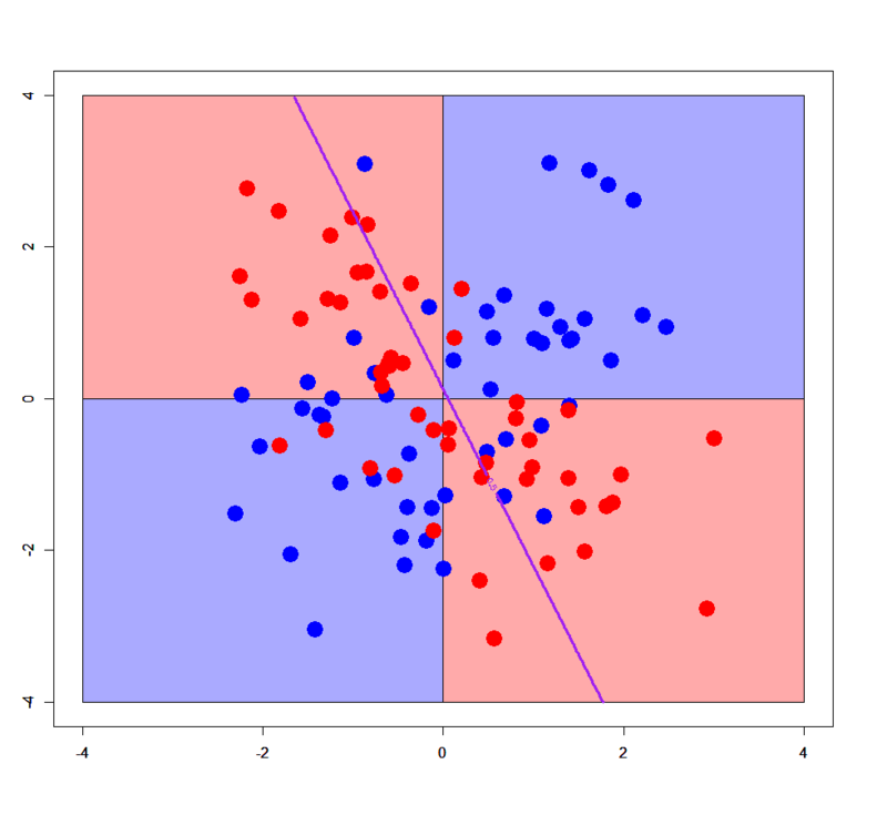
Of course logistic regression cannot classify correctly for any XOR patterns. But in some limited cases it works even for such a linearly non-separable pattern. See below.

# Just added an interaction term
> xors.glm2<-glm(label~x+y+x:y,xors,family=binomial)
> xorc.glm2<-glm(label~x+y+x:y,xorc,family=binomial)
# Plot for simple XOR
> plot(c(),type='n',xlim=c(-4,4),ylim=c(-4,4))
> par(new=T)
> rect(0,0,4,4,col='#aaaaff')
> par(new=T)
> rect(-4,0,0,4,col='#ffaaaa')
> par(new=T)
> rect(-4,-4,0,0,col='#aaaaff')
> par(new=T)
> rect(0,-4,4,0,col='#ffaaaa')
> par(new=T)
> plot(xors[,-3],col=c(rep('blue',50),rep('red',50)),xlim=c(-4,4),ylim=c(-4,4),pch=19,cex=2.5)
> par(new=T)
> contour(px,py,array(predict(xors.glm2,newdata=pgrid,type='response'),dim = c(length(px),length(py))),levels = 0.5,drawlabels = T,col='purple',lwd=3,xlim=c(-4,4),ylim=c(-4,4))
# Plot for complex XOR
> plot(c(),type='n',xlim=c(-4,4),ylim=c(-4,4))
> par(new=T)
> rect(0,0,4,4,col='#aaaaff')
> par(new=T)
> rect(-4,0,0,4,col='#ffaaaa')
> par(new=T)
> rect(-4,-4,0,0,col='#aaaaff')
> par(new=T)
> rect(0,-4,4,0,col='#ffaaaa')
> par(new=T)
> plot(xorc[,-3],col=c(rep('blue',50),rep('red',50)),xlim=c(-4,4),ylim=c(-4,4),pch=19,cex=2.5)
> par(new=T)
> contour(px,py,array(predict(xorc.glm2,newdata=pgrid,type='response'),dim = c(length(px),length(py))),levels = 0.5,drawlabels = T,col='purple',lwd=3,xlim=c(-4,4),ylim=c(-4,4))

f:id:TJO:20150325174020p:plain

f:id:TJO:20150325174032p:plain

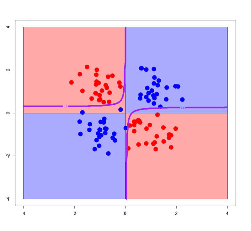
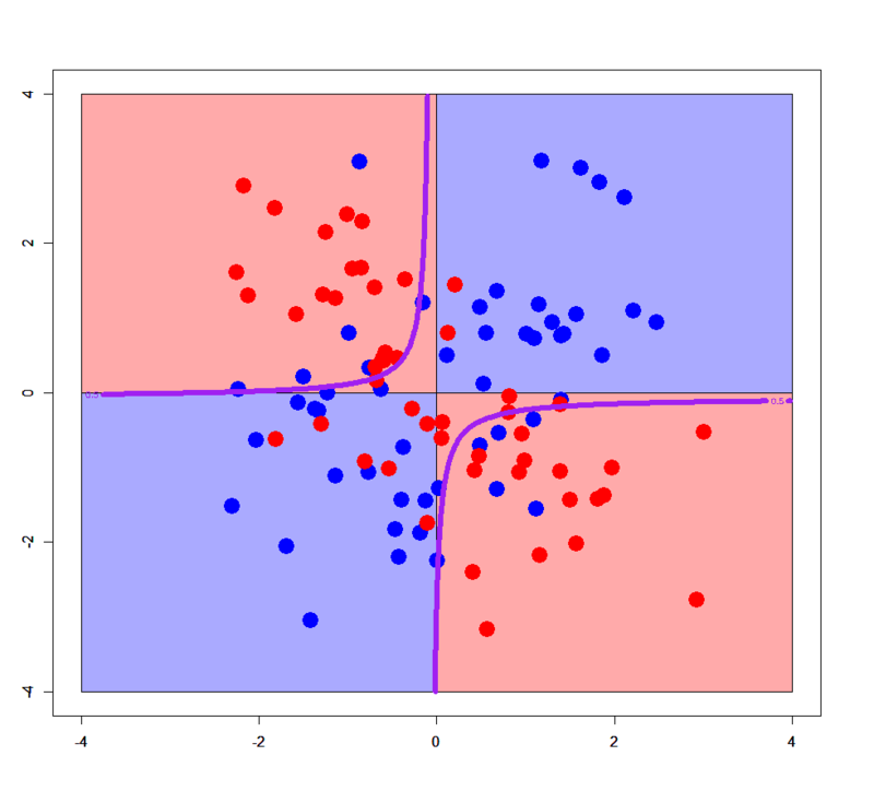
In this case an interaction term $z = xy$ help it classify samples. You can easily see in 3D space how it works.

> library(scatterplot3d)
> par(mfrow=c(1,2))
> scatterplot3d(xors$x,xors$y,xors$x*xors$y,color=c(rep('blue',50),rep('red',50)),pch=19,cex.symbols = 2)
> scatterplot3d(xors$x,xors$y,xors$x*xors$y,color=c(rep('blue',50),rep('red',50)),pch=19,cex.symbols = 2,angle = 0)
> scatterplot3d(xorc$x,xorc$y,xorc$x*xorc$y,color=c(rep('blue',50),rep('red',50)),pch=19,cex.symbols = 2)
> scatterplot3d(xorc$x,xorc$y,xorc$x*xorc$y,color=c(rep('blue',50),rep('red',50)),pch=19,cex.symbols = 2,angle = 0)

f:id:TJO:20150325174813p:plain

f:id:TJO:20150325174823p:plain

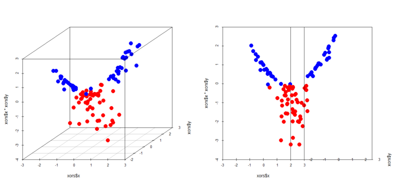
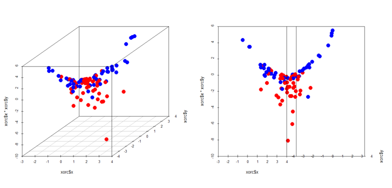
Yes, in both cases a plain $z=0$ well classifies the samples. This is just a specific case but it's important to remember this characteristic of logistic regression.

Linearly separable patterns

We know logistic regression obviously works well for linearly separable patterns, but it's important to see how good really it works. Please download "linear_bi.txt" and "linear_multi.txt" from my GitHub repository and import them.

> dbi<-read.table("linear_bi.txt",header=T)
> dml<-read.table("linear_multi.txt",header=T)
> dbi$label<-as.factor(dbi$label)
> dml$label<-as.factor(dml$label)
> px2<-seq(-0.5,4.5,0.1)
> py2<-seq(-0.5,4.5,0.1)
> pgrid2<-expand.grid(px2,py2)
> names(pgrid2)<-names(dbi)[-3]

OK, let's run as below.

# 2-classes: binomial logit
> dbi.glm<-glm(label~.,dbi,family=binomial)

# 3-classes: multinomial logit
> library(VGAM)
> dml.vglm<-vglm(label~.,dml,family=multinomial)
> out.vglm<-predict(dml.vglm,newdata=pgrid2,type="response")
> out.vglm.class<-matrix(rep(0,dim(out.vglm)[1]),ncol=1)
> for (i in 1:length(out.vglm.class)) {
+     out.vglm.class[i]<-as.numeric(which.max(out.vglm[i,]))-1
+ }

# Plot with binomial logit
> plot(c(),type='n',xlim=c(-0.5,3.5),ylim=c(-0.5,3.5))
> par(new=T)
> polygon(c(-0.5,-0.5,3.5),c(3.5,-0.5,-0.5),col='#aaaaff')
> par(new=T)
> polygon(c(-0.5,3.5,3.5),c(3.5,-0.5,3.5),col='#ffaaaa')
> par(new=T)
> plot(dbi[,-3],pch=19,col=c(rep('blue',25),rep('red',25)),cex=3,xlim=c(-0.5,3.5),ylim=c(-0.5,3.5))
> par(new=T)
> contour(px2,py2,array(predict(dbi.glm,newdata=pgrid2),dim = c(length(px2),length(py2))),xlim=c(-0.5,3.5),ylim=c(-0.5,3.5),lwd=6,col='purple',levels = 0.5,drawlabels = T)

# Plot with multinomial logit
> plot(c(),type='n',xlim=c(-0.5,4.5),ylim=c(-0.5,4.5))
> par(new=T)
> polygon(c(-0.5,-0.5,3.5),c(3.5,-0.5,-0.5),col='#aaaaff')
> par(new=T)
> polygon(c(-0.5,3.5,4.5,4.5,1.0,-0.5),c(3.5,-0.5,-0.5,1.0,4.5,4.5),col='#ffaaaa')
> par(new=T)
> polygon(c(1.0,4.5,4.5),c(4.5,1.0,4.5),col='#ccffcc')
> par(new=T)
> plot(dml[,-3],pch=19,col=c(rep('blue',25),rep('red',25),rep('green',25)),cex=3,xlim=c(-0.5,4.5),ylim=c(-0.5,4.5))
> par(new=T)
> contour(px2,py2,array(out.vglm.class,dim=c(length(px2),length(py2))),xlim=c(-0.5,4.5),ylim=c(-0.5,4.5),col="purple",lwd=6,drawlabels=T,levels=c(0.5,1.5))

f:id:TJO:20150402174435p:plain

f:id:TJO:20150402174446p:plain

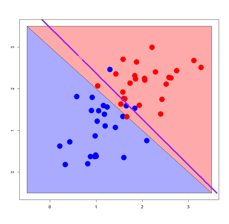
All perfect! :) Please remember how decision tree works on the same linearly separable patterns.

f:id:TJO:20150320190847p:plain:w250 f:id:TJO:20150320190901p:plain:w250

Conclusions

Lessons in this post are:

Logistic regression is one of the best classifier for linearly separable patterns
But in some limited cases it also works for linearly non-separable patterns with some interaction terms

Actually I don't know how interaction terms strictly work in logistic regression (in particular its theoretical property), but I think it would be helpful for improving performance of logistic regression as a classifier.