Bayesian modeling with R and Stan (5): Time series with seasonality

In the previous post, we successfully estimated a model with a nonlinear trend by using Stan.

But please remember this is a time series dataset. Does it include any other kind of nonlinear components? Yes, we have to be careful for seasonality. Actually when I generate the dataset, I added a seasonal component with a 7 days cycle.

Then we have to change the model as follows.

The model above can be described with a Stan code below. Save it as "hb_ts2.stan".

data {
	int<lower=0> N;
	real<lower=0> x1[N];
	real<lower=0> x2[N];
	real<lower=0> x3[N];
	real<lower=0> y[N];
}

parameters {
	real trend[N];
	real season[N];
	real s_trend;
	real s_q;
	real s_season;
	real<lower=0> a;
	real<lower=0> b;
	real<lower=0> c;
	real d;
}

model {
	real q[N];
	real cum_trend[N];
	for (i in 7:N) {
		season[i]~normal(-season[i-1]-season[i-2]-season[i-3]-season[i-4]-season[i-5]-season[i-6],s_season);
	}
	for (i in 3:N)
		trend[i]~normal(2*trend[i-1]-trend[i-2],s_trend);
	cum_trend[1]<-trend[1];
	for (i in 2:N)
		cum_trend[i]<-cum_trend[i-1]+trend[i];

	for (i in 1:N)
		q[i]<-y[i]-cum_trend[i]-season[i];
	for (i in 1:N)
		q[i]~normal(a*x1[i]+b*x2[i]+c*x3[i]+d,s_q);
}

Are you ready? Now just run as below. It may take much long time because computing seasonality is heavy, so please be patient :)

> fit2<-stan(file='hb_ts2.stan',data=dat,iter=1000,chains=4)
> fit2.smp<-extract(fit2)
> dens2_a<-density(fit2.smp$a)
> dens2_b<-density(fit2.smp$b)
> dens2_c<-density(fit2.smp$c)
> dens2_d<-density(fit2.smp$d)
> a_est2<-dens2_a$x[dens2_a$y==max(dens2_a$y)]
> b_est2<-dens2_b$x[dens2_b$y==max(dens2_b$y)]
> c_est2<-dens2_c$x[dens2_c$y==max(dens2_c$y)]
> d_est2<-dens2_d$x[dens2_d$y==max(dens2_d$y)]
> trend_est2<-rep(0,100)
> for (i in 1:100) {
+     tmp<-density(fit2.smp$trend[,i])
+     trend_est2[i]<-tmp$x[tmp$y==max(tmp$y)]
+ }
> week_est2<-rep(0,100)
> for (i in 1:100) {
+     tmp<-density(fit2.smp$season[,i])
+     week_est2[i]<-tmp$x[tmp$y==max(tmp$y)]
+ }
> pred2<-a_est2*d$x1+b_est2*d$x2+c_est2*d$x3+d_est2+cumsum(trend_est2)+week_est2
> matplot(cbind(d$y,pred2),type='l',lty=1,lwd=c(2,3),col=c(1,2))
> legend('topleft',c('Data','Predicted'),col=c(1,2),lty=1,lwd=c(2,3),cex=1.5,ncol=2)
> cor(d$y,pred)
[1] 0.9452432
> cor(d$y,pred2)
[1] 0.9949925

Perfect! Just for your information, plot its seasonal component.

> plot(week_est2,type='l')

It's a precise 7-days cycle. Parameters are also well estimated, better than without seasonality.

> a_est2
[1] 0.0001505969
> b_est2
[1] 0.0002937902
> c_est2
[1] 5.39804e-05
> d_est2
[1] 1516.145

The only failure is an intercept because it can be included in the other components such as trend or seasonality. I have no idea for solving it but it doesn't matter I think.

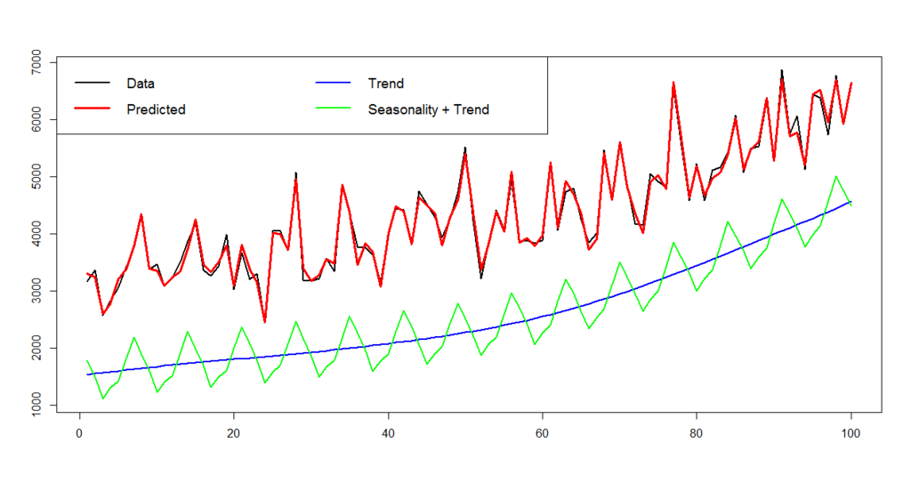
Finally, just plot as below.

> matplot(cbind(d$y,pred2,cumsum(trend_est2)+d_est2,week_est2+cumsum(trend_est2)+d_est2),type='l',lty=1,lwd=c(2,3,2,2),col=c('black','red','blue','green'))
> legend('topleft',c('Data','Predicted','Trend','Seasonality + Trend'),col=c('black','red','blue','green'),lty=1,lwd=c(2,3,2,2),cex=1.2,ncol=2)

A trend and seasonality are decomposed and visualized.

Conclusions

The lessons we learn in these 2 posts are:

1. A time series with a nonlinear trend cannot be precisely modeled by usual linear regression
2. As well as dynamic linear modeling or state-space modeling, Bayesian modeling with MCMC can model it
3. In case of usual econometric time series analysis, you have to be careful for seasonality

In some extreme cases a time series may contain further complicated nonlinear components such as weekend effect, ultra-long term trend, etc. But Bayesian modeling can handle them with its great flexibility.